
Simultaneous and semi-alternating projection algorithms for solving split equality problems

Abstract

In this article, we first introduce two simultaneous projection algorithms for solving the split equality problem by using a new choice of the stepsize, and then propose two semi-alternating projection algorithms. The weak convergence of the proposed algorithms is analyzed under standard conditions. As applications, we extend the results to solve the split feasibility problem. Finally, a numerical example is presented to illustrate the efficiency and advantage of the proposed algorithms.

1 Introduction

Let \(H_{1}\), \(H_{2}\) and \(H_{3}\) be real Hilbert spaces, let \(C \subseteq H_{1}\) and \(Q \subseteq H_{2}\) be two nonempty closed convex sets, and let \(A: H_{1}\rightarrow H_{3}\) and \(B: H_{2} \rightarrow H_{3}\) be two bounded linear operators.

In this article, we consider the classical split equality problem (SEP), which was first introduced by Moudafi [1]. The SEP can mathematically be formulated as follows:

$$ \mbox{Find}\quad x \in C, y \in Q \quad \mbox{such that} \quad Ax=By . $$
(1)

Throughout this paper, assume that SEP (1) is consistent and denote by

$$\Gamma=\{ x\in C,y\in Q: Ax=By\} $$

the solution of SEP (1). Then Γ is closed, convex and nonempty.

The split equality problem (1) is actually an optimization problem with weak coupling in the constraint (see [1] for details) and its interest covers many situations, for instance, in domain decomposition for PDEs, game theory and intensity-modulated radiation therapy (IMRT). In domain decomposition for PDEs, this equals to the variational form of a PDE in a domain that can be decomposed into two non-overlapping subdomains with a common interface (see, e.g., [2]). In decision sciences, this allows to consider agents who interplay only via some components of their decision variables (see, e.g., [3]). In IMRT, this amounts to envisaging a weak coupling between the vector of doses absorbed in all voxels and that of the radiation intensity (see [4] for further details). Attouch [5] pointed out more applications of the SEP in optimal control theory, surface energy and potential games, whose variational form can be seen as a SEP.

Next we present an example, in which a separable optimization problem can be rewritten as a split equality problem.

Example 1.1

Consider the separable optimization problem

$$ \begin{aligned} &\mbox{minimize } f(x)+g(y) \\ &\quad \mbox{subject to } Ax=By, \end{aligned} $$
(2)

with \(x \in R^{N}\) and \(y \in R^{M}\), where \(A\in R^{J\times N}\) and \(B\in R^{J\times M}\). Assume that f and g are convex and the solution set of problem (2) is nonempty.

Set \(C=\operatorname*{argmin}\{f(x) \mid x\in R^{N} \}\) and \(Q=\operatorname*{argmin}\{g(y) \mid y\in R^{M} \}\). Then the optimization problem (2) equals to the following split equality problem:

$$ \mbox{Find}\quad x \in C, y \in Q \quad \mbox{such that} \quad Ax=By. $$
(3)

A great deal of literature on algorithms for solving SEP has been published, most of which are projection methods [13, 611]. Based on the classical projection gradient algorithm, Byrne and Moudafi [12] introduced the following algorithm, which is also called the simultaneous iterative method [13]:

$$ \textstyle\begin{cases} x^{k+1}=P_{C}(x^{k}-\beta_{k} A^{*}( A x^{k}-B y^{k})), \\ y^{k+1}=P_{Q}(y^{k}+\beta_{k} B^{*}(A x^{k}-B y^{k})), \end{cases} $$
(4)

where \(\beta_{k}\in(\varepsilon,{2}/({\lambda_{A}+\lambda _{B}})-\varepsilon)\), \(\lambda_{A}\) and \(\lambda_{B}\) are the operator (matrix) norms \(\|A\|\) and \(\|B\|\) (or the largest eigenvalues of \(A^{*}A\) and \(B^{*}B\)), respectively. To determine stepsize \(\beta_{k}\), one needs first to calculate (or estimate) the operator norms \(\|A\|\) and \(\|B\|\). In general, it is difficult or even impossible. On the other hand, even if we know the norm of A and B, the algorithm (4) method with fixed stepsize may be slow.

In order to deal with this, the authors [9] introduced a self-adaptive projection algorithm, in which the stepsize is computed by using an Armijo search.

Define the function \(F:H_{1}\times H_{2} \rightarrow H_{1}\) by

$$F(x,y)=A^{*}(Ax-By), $$

and the function \(G:H_{1}\times H_{2} \rightarrow H_{2}\) by

$$G(x,y)=B^{*}(By-Ax). $$

The self-adaptive projection algorithm in [9] is defined as follows.

Algorithm 1.1

Given constants \(\sigma_{0} > 0\), \(\alpha\in(0, 1)\), \(\theta\in(0, 1)\) and \(\rho\in(0,1)\). Let \(x^{0}\in H_{1}\) and \(y^{0}\in H_{2}\) be taken arbitrarily. For \(k=0,1,2,\ldots\) , compute

$$ \textstyle\begin{cases} u^{k}=P_{C}(x^{k}-\beta_{k}F(x^{k},y^{k})), \\ v^{k}=P_{Q}(y^{k}-\beta_{k}G(x^{k},y^{k})), \end{cases} $$
(5)

where \(\beta_{k}\) is chosen to be the largest \(\beta\in\{\sigma_{k},\sigma _{k}\alpha,\sigma_{k}\alpha^{2},\ldots\}\) satisfying

$$\begin{aligned}& {\beta^{2}}\bigl( \bigl\Vert F\bigl(x^{k},y^{k} \bigr)-F\bigl(u^{k},v^{k}\bigr) \bigr\Vert ^{2}+ \bigl\Vert G\bigl(x^{k},y^{k}\bigr)-G\bigl(u^{k},v^{k} \bigr) \bigr\Vert ^{2}\bigr) \\& \quad \leq \theta^{2}\bigl({ \bigl\Vert x^{k}-u^{k} \bigr\Vert ^{2}+ \bigl\Vert y^{k}-v^{k} \bigr\Vert ^{2}}\bigr). \end{aligned}$$
(6)

Compute

$$ \textstyle\begin{cases} x^{k+1}=P_{C}(x^{k}-\beta_{k}F(u^{k},v^{k})), \\ y^{k+1}=P_{Q}(y^{k}-\beta_{k}G(u^{k},v^{k})). \end{cases} $$
(7)

If

$$\begin{aligned}& {\beta_{k}^{2}}\bigl( \bigl\Vert F\bigl(x^{k},y^{k} \bigr)-F\bigl(x^{k+1},y^{k+1}\bigr) \bigr\Vert ^{2}+ \bigl\Vert G\bigl(x^{k},y^{k}\bigr)-G\bigl(x^{k+1},y^{k+1} \bigr) \bigr\Vert ^{2}\bigr) \\& \quad \leq\rho^{2}\bigl({ \bigl\Vert x^{k}-x^{k+1} \bigr\Vert ^{2}+ \bigl\Vert y^{k}-y^{k+1} \bigr\Vert ^{2}}\bigr), \end{aligned}$$
(8)

then set \(\sigma_{k}=\sigma_{0}\); otherwise, set \(\sigma_{k}=\beta_{k}\).

In fact, Algorithm 1.1 can be seen as an extension of the classical extragradient method first proposed by Korpelevich [14]. Notice that, in Algorithm 1.1, the stepsize of the prediction (5) and that of the correction (7) are equal. Thus these two steps seem to be ‘symmetric’.

Recently, Chuang and Du [15] proposed the following projection algorithm (which is called the hybrid projected Landweber algorithm).

Algorithm 1.2

Given constants \(\sigma>0, \alpha\in(0,1)\) and \(\theta\in(0,1)\), let \(x^{0} \in H_{1}\) and \(y^{0}\in H_{2}\) be taken arbitrarily. For \(k = 0,1,2,\ldots \) , compute

$$\textstyle\begin{cases} u^{k}=P_{C}(x^{k}-\beta_{k} F(x^{k},y^{k})), \\ v^{k}=P_{Q}(y^{k}-\beta_{k} G(x^{k},y^{k})), \end{cases} $$

where \(\beta_{k}\) is chosen via (6) and (8). Compute next iterates \(x^{k+1}\) and \(y^{k+1}\) by

$$ \textstyle\begin{cases} x^{k+1}=P_{C}(x^{k}-\rho_{k} c_{k}), \\ y^{k+1}=P_{Q}(y^{k}-\rho_{k} d_{k}), \end{cases} $$
(9)

where

$$\textstyle\begin{cases} c_{k}:=(x^{k}-u^{k})-\beta_{k}(F(x^{k},y^{k})-F(u^{k},v^{k})); \\ d_{k}:=(y^{k}-v^{k})-\beta_{k}(G(x^{k},y^{k})-G(u^{k},v^{k})), \end{cases} $$

and

$$ \rho_{k}:=\frac{\langle x^{k}-u^{k}, c_{k}\rangle+\langle y^{k}-v^{k}, d_{k}\rangle }{\|c_{k}\|^{2}+\|d_{k}\|^{2}}. $$
(10)

Note that Algorithm 1.2 with \(\rho_{k}\equiv1\) in (9) can be seen as a special case of Tseng’s method [8, 16]. The projections in the second step of Tseng’s method are made onto two nonempty closed convex sets \(X\subseteq H_{1}\) and \(Y\subseteq H_{2}\), other than C and Q. X and Y can be any sets such that the intersections of X and C (and Y and Q) are nonempty, and they may be taken to have simple structures so that the projections onto them are easy to calculate.

Chuang and Du [15] proved the convergence of Algorithm 1.2 and also presented the convergence property of Algorithm 1.2 as follows:

$$\begin{aligned}& \bigl\Vert x^{k+1}-x^{*} \bigr\Vert ^{2}+ \bigl\Vert y^{k+1}-y^{*} \bigr\Vert ^{2} \\& \quad \leq \bigl\Vert x^{k}-x^{*} \bigr\Vert ^{2}+ \bigl\Vert y^{k}-y^{*} \bigr\Vert ^{2}-\rho_{k}^{2} \bigl( \Vert c_{k} \Vert ^{2}+ \Vert d_{k} \Vert ^{2}\bigr), \end{aligned}$$
(11)

where \((x^{*},y^{*})\in\Gamma\).

The stepsize \(\beta_{k}\) in Algorithms 1.1 and 1.2 is obtained through the Armijo search (6). In general, the computational cost of a self-adaptive algorithm is large, since one may need to calculate (5) several times to get the stepsize \(\beta_{k}\).

To overcome this difficulty, the authors [17] introduced a projection algorithm for which the stepsize does not depend on the operator norms \(\|A\|\) and \(\|B\|\), and one can directly compute the stepsize instead of using the Armijo search.

Algorithm 1.3

Choose initial guesses \(x^{0}\in H_{1}, y^{0}\in H_{2}\) arbitrarily. Assume that the kth iterate \(x^{k} \in C\), \(y^{k}\in Q\) has been constructed and \(Ax^{k}-By^{k}\neq0\); then we calculate the \((k + 1)\)th iterate \((x^{k+1},y^{k+1})\) via the formula

$$ \textstyle\begin{cases} x^{k+1}=P_{C}(x^{k}-\beta_{k} A^{*}(Ax^{k}-By^{k})), \\ y^{k+1}=P_{Q}(y^{k}+\beta_{k} B^{*}(Ax^{k}-By^{k})), \end{cases} $$
(12)

where the stepsize \(\beta_{k}\) is chosen in such a way that

$$ \beta_{k}=\sigma_{k}\min \biggl\{ \frac{ \Vert Ax^{k}-By^{k} \Vert ^{2}}{ \Vert A^{*}(Ax^{k}-By^{k}) \Vert ^{2}}, \frac{ \Vert Ax^{k}-By^{k} \Vert ^{2}}{ \Vert B^{*}(Ax^{k}-By^{k}) \Vert ^{2}} \biggr\} , $$
(13)

where \(0<\sigma_{k}<1\). If \(Ax^{k}-By^{k}= 0\), then \((x^{k+1},y^{k+1})=(x^{k},y^{k})\) is a solution of SEP (1) and the iterative process stops; otherwise, we set \(k := k + 1\) and go onto (12) to evaluate the next iterate \((x^{k+2},y^{k+2})\).

Note that the choice in (13) of the stepsize \(\beta_{k}\) is independent of the norms \(\|A\|\) and \(\|B\|\).

Polyak [18, 19] first introduced the inertial extrapolation algorithms, which were widely studied as an acceleration process. The authors [20] made an inertial modification for Algorithm 1.3 and introduced the following inertial projection methods for SEP.

Algorithm 1.4

Choose initial guesses \(x^{0},x^{1}\in H_{1}\), \(y^{0},y^{1}\in H_{2}\) arbitrarily. Compute

$$ \textstyle\begin{cases} (\bar{x}^{k},\bar{y}^{k})=(x^{k},y^{k})+\alpha_{k}(x^{k}-x^{k-1},y^{k}-y^{k-1}), \\ x^{k+1}=P_{C}(\bar{x}^{k}-\beta_{k} A^{*}( A\bar{x}^{k}-B\bar{y}^{k})), \\ y^{k+1}=P_{Q}(\bar{y}^{k}+\beta_{k}B^{*}(A\bar{x}^{k}-B\bar{y}^{k})), \end{cases} $$
(14)

where \(\alpha_{k}\in(0,1)\) and the stepsize \(\gamma_{k}\) is chosen in the same way as (13).

They showed the weak convergence of Algorithm 1.4 under some conditions on the inertial parameter \(\alpha_{k}\).

In fact, Algorithm 1.4 can be seen as a FISTA (fast iterative shrinkage-thresholding algorithm) introduced by Beck and Teboulle [21] to solve the linear inverse problems, if we take the inertial parameter \(\alpha_{k}=\frac{t_{k}-1}{t_{k+1}}\), where \(t_{1}=1\) and \(t_{k+1}=\frac{1+\sqrt{1+4t_{k}^{2}}}{2}\), \(k\geq1 \), and choose a constant stepsize \(\beta_{k}\) or choose \(\beta_{k}\) via a backtracking stepsize rule. A shortcoming of the method of Beck and Teboulle is that they could not prove the convergence of the iterative sequence \((x^{k},y^{k})\). Chambolle and Dossal [22] improved the choice of the inertial parameter, took \(\alpha_{k}=\frac{k-1}{k+a}\), where \(a>2\), and presented the convergence of the iterative sequence \((x^{k},y^{k})\).

In this paper, inspired by the work in [17, 23, 24], we introduce two simultaneous projection algorithms by improving the stepsizes \(\beta_{k}\) and \(\rho_{k}\) of the second step (7) and (9) in Algorithms 1.1 and 1.2, respectively. We also present two alternating projection algorithms, in which we take an alternating technique in the first step.

The structure of the paper is as follows. In the next section, we present some concepts and lemmas which will be used in the main results. In Section 3, two classes of projection algorithms are provided and their weak convergence is analyzed. In Section 4, we extend the results to the split feasibility problem. In the final section, some numerical results are provided, which show the advantages of the proposed algorithms.

2 Preliminaries

Let H be a real Hilbert space with the inner product \(\langle\cdot ,\cdot\rangle\) and the induced norm \(\Vert\cdot\Vert\), and let D be a nonempty, closed and convex subset of H. We write \(x^{k}\rightharpoonup x\) to indicate that the sequence \(\{ x^{k} \} _{k=0}^{\infty}\) converges weakly to x and \(x^{k}\rightarrow x\) to indicate that the sequence \(\{ x^{k} \} _{k=0}^{\infty}\) converges strongly to x. Given a sequence \(\{ x^{k} \} _{k=0}^{\infty}\), denote by \(\omega_{w}(x^{k})\) its weak ω-limit set, that is, any \(x\in\omega_{w}(x^{k})\) such that there exists a subsequence \(\{ x^{k_{j}} \} _{j=0}^{\infty}\) of \(\{ x^{k} \} _{k=0}^{\infty}\) which converges weakly to x.

In this paper, an important tool of our work is the projection. Let H be a real Hilbert space and C be a closed convex subset of H. Recall that the projection from H onto C, denoted by \(P_{C}\), is defined in such a way that, for each \(x\in H\), \(P_{C}(x)\) is the unique point in C such that

$$\bigl\Vert x-P_{C}(x) \bigr\Vert =\min\bigl\{ \Vert x-z \Vert :z\in C\bigr\} . $$

The following two lemmas are useful characterizations of projections.

Lemma 2.1

([25])

Given \(x\in H\) and \(z\in C\). Then \(z=P_{C}(x)\) if and only if

$$\langle x-z,y-z\rangle\leq0,\quad \forall y\in C. $$

Lemma 2.2

([25, 26])

For any \(x,y\in H\) and \(z\in C\), it holds

  1. (i)

    \(\|P_{C}(x)-P_{C}(y)\|\leq\|x-y\|\);

  2. (ii)

    \(\|P_{C}(x)-z\|^{2}\leq\|x-z\|^{2}-\|P_{C}(x)-x\|^{2}\).

Definition 2.1

The normal cone of C at \(v\in C\), denoted by \(N_{C} ( v )\), is defined as

$$N_{C} ( v ) :=\bigl\{ d\in H\mid \langle d,y-v \rangle\leq0\text{ for all }y\in C\bigr\} . $$

Definition 2.2

Let \(A:H\rightrightarrows2^{H}\) be a point-to-set operator defined on a real Hilbert space H. The operator A is called a maximal monotone operator if A is monotone, i.e.,

$$\langle u-v,x-y \rangle\geq0\quad \text{for all }u\in A(x)\text{ and }v\in A(y), $$

and the graph \(G(A)\) of A,

$$G(A):= \bigl\{ ( x,u ) \in H\times H\mid u\in A(x) \bigr\} , $$

is not properly contained in the graph of any other monotone operator.

It is clear [27, Theorem 3] that a monotone mapping A is maximal if and only if, for any \(( x,u ) \in H\times H\), if \(\langle u-v,x-y \rangle\geq0\) for all \(( v,y ) \in G(A)\), then it follows that \(u\in A(x)\).

Lemma 2.3

([26])

Let D be a nonempty, closed and convex subset of a Hilbert space H. Let \((x^{k})\) be a bounded sequence which satisfies the following properties:

  1. (i)

    every limit point of \(\{x^{k}\}_{k=0}^{\infty}\) lies in D;

  2. (ii)

    \(\lim_{n\rightarrow\infty}\Vert x^{k}-x\Vert\) exists for every \(x\in D\).

Then \(\{x^{k}\}\) converges weakly to a point in D.

3 Main results

In this section, we present two classes of projection algorithms and establish their weak convergence under standard conditions.

3.1 Simultaneous projection algorithms

Let \(S= C\times Q\in H := H_{1}\times H_{2}\). Define \(K =[A,-B] : H_{1} \times H_{2} \rightarrow H_{1} \times H_{2}\), and let \(K^{*}\) be the adjoint operator of K, then the original problem (1) can be modified as

$$ \mbox{Find} \quad z=(x,y)\in S \quad \mbox{such that} \quad Kw=0. $$
(15)

Note that if the solution set of (15) is nonempty, it equals the following minimization problem:

$$ \min_{z\in S}\frac{1}{2}\|Kz \|^{2}, $$
(16)

which is a standard (and a simple) problem from the convex optimization point of view. There are many methods for solving the minimization problem (16) such as the classical projection gradient method. Algorithm (4) (also Algorithm 1.3) is the exact projection gradient method when applied to (16).

Inspired by Cai [24] and Dong et al. [17], we propose two new simultaneous projection algorithms by improving the stepsizes in the second step of Algorithms 1.1 and 1.2.

Algorithm 3.1

Given constants \(\sigma>0\), \(\alpha\in(0,1)\), \(\theta\in(0,1)\) and \(\rho\in(0,1)\), let \(z_{0}=(x^{0},y^{0}) \in H=H_{1}\times H_{2}\) be taken arbitrarily.

For \(k = 0,1,2,\ldots \) , compute

$$ w^{k}=P_{S}\bigl(z^{k}- \beta_{k} K^{*}K\bigl(z^{k}\bigr)\bigr), $$
(17)

where \(\beta_{k}\) is chosen to be the largest \(\beta\in\{\sigma_{k},\sigma _{k}\alpha,\sigma_{k}\alpha^{2},\ldots \}\) satisfying

$$ \beta \bigl\Vert K^{*}K\bigl(z^{k}\bigr)-K^{*}K \bigl(w^{k}\bigr) \bigr\Vert \leq\theta \bigl\Vert z^{k}-w^{k} \bigr\Vert . $$
(18)

Compute next iterates \(z^{k+1}\) by

$$ z^{k+1}_{\mathrm{I}}=z^{k}-\gamma \rho_{k} d\bigl(z^{k},w^{k}\bigr), $$
(19)

or

$$ z^{k+1}_{\mathrm{II}}=P_{S} \bigl(z^{k}-\gamma\beta_{k}\rho_{k} K^{*}K \bigl(w^{k}\bigr)\bigr), $$
(20)

where \(\gamma\in[0,2)\),

$$ d\bigl(z^{k},w^{k}\bigr):= \bigl(z^{k}-w^{k}\bigr)-\beta_{k}\bigl(K^{*}K \bigl(z^{k}\bigr)-K^{*}K\bigl(w^{k}\bigr)\bigr), $$
(21)

and

$$ \rho_{k}:=\frac{\langle z^{k}-w^{k}, d(z^{k},w^{k})\rangle+\beta_{k} \Vert K(w^{k}) \Vert ^{2}}{ \Vert d(z^{k},w^{k}) \Vert ^{2}}. $$
(22)

If

$$ \beta_{k} \bigl\Vert K^{*}K\bigl(z^{k} \bigr)-K^{*}K\bigl(z^{k+1}\bigr) \bigr\Vert \leq\rho \bigl\Vert z^{k}-z^{k+1} \bigr\Vert , $$
(23)

then set \(\sigma_{k}=\sigma_{0}\); otherwise, set \(\sigma_{k}=\beta_{k}\).

Remark 3.1

Let \(z=(x,y)\). Then we have (see Section 4.4.1 in [28])

$$P_{S}(z)=(P_{C}x,P_{Q}y). $$

It is easy to see

$$K^{*}Kz= \left ( \textstyle\begin{array}{@{}c@{\quad}c@{}} A^{*}A&-A^{*}B\\ -B^{*}A&B^{*}B \end{array}\displaystyle \right ) \left ( \textstyle\begin{array}{@{}c@{}} x\\ y \end{array}\displaystyle \right ) = \left ( \textstyle\begin{array}{@{}c@{}} A^{*}(Ax-By)\\ B^{*}(By-Ax) \end{array}\displaystyle \right ). $$

Define the function \(F: H_{1} \times H_{2} \rightarrow H_{1}\) by

$$ F(x,y)=A^{*}(Ax-By), $$
(24)

and the function \(G: H_{1} \times H_{2} \rightarrow H_{2}\) by

$$ G(x,y)=B^{*}(By-Ax). $$
(25)

By setting \(z^{k}=(x^{k},y^{k})\) and \(w^{k}=(u^{k},v^{k})\), Algorithm 3.1 can be rewritten as follows:

For \(k = 0,1,2,\ldots \) , compute

$$ \textstyle\begin{cases} u^{k}=P_{C}(x^{k}-\beta_{k} F(x^{k},y^{k})),\\ v^{k}=P_{Q}(y^{k}-\beta_{k} G(x^{k},y^{k})), \end{cases} $$
(26)

where \(\beta_{k}\) is chosen to be the largest \(\beta\in\{\sigma_{k},\sigma _{k}\alpha,\sigma_{k}\alpha^{2},\ldots \}\) satisfying

$$\begin{aligned}& \beta^{2}\bigl( \bigl\Vert F\bigl(x^{k},y^{k} \bigr)-F\bigl(u^{k},v^{k}\bigr) \bigr\Vert ^{2}+ \bigl\Vert G\bigl(x^{k},y^{k}\bigr)-G\bigl(u^{k},v^{k} \bigr) \bigr\Vert ^{2}\bigr) \\& \quad \leq \theta^{2}\bigl( \bigl\Vert x^{k}-u^{k} \bigr\Vert ^{2}+ \bigl\Vert y^{k}-v^{k} \bigr\Vert ^{2}\bigr). \end{aligned}$$
(27)

Compute next iterates \(x^{k+1}\) and \(y^{k+1}\) by

$$ \textstyle\begin{cases} x^{k+1}_{\mathrm{I}}=x^{k}-\gamma\rho_{k} c_{k}, \\ y^{k+1}_{\mathrm{I}}=y^{k}-\gamma\rho_{k} d_{k}, \end{cases} $$
(28)

or

$$ \textstyle\begin{cases} x^{k+1}_{\mathrm{II}}=P_{C}(x^{k}-\gamma\beta _{k}\rho_{k} F(u^{k},v^{k})), \\ y^{k+1}_{\mathrm{II}}=P_{Q}(y^{k}-\gamma\beta _{k}\rho_{k} G(u^{k},v^{k})), \end{cases} $$
(29)

where \(\gamma\in[0,2)\),

$$ \textstyle\begin{cases} c_{k}:=(x^{k}-u^{k})-\beta_{k}(F(x^{k},y^{k})-F(u^{k},v^{k})); \\ d_{k}:=(y^{k}-v^{k})-\beta_{k}(G(x^{k},y^{k})-G(u^{k},v^{k})), \end{cases} $$
(30)

and

$$ \begin{aligned}\rho_{k}:=\frac{\langle x^{k}-u^{k}, c_{k}\rangle+\langle y^{k}-v^{k}, d_{k}\rangle +\beta_{k}\| Au^{k}-Bv^{k}\|^{2}}{\|c_{k}\|^{2}+\|d_{k}\|^{2}}.\end{aligned}$$
(31)

If

$$\begin{aligned}& {\beta_{k}^{2}}\bigl( \bigl\Vert F\bigl(x^{k},y^{k} \bigr)-F\bigl(x^{k+1},y^{k+1}\bigr) \bigr\Vert ^{2}+ \bigl\Vert G\bigl(x^{k},y^{k}\bigr)-G\bigl(x^{k+1},y^{k+1} \bigr) \bigr\Vert ^{2}\bigr) \\& \quad \leq\rho^{2}\bigl({ \bigl\Vert x^{k}-x^{k+1} \bigr\Vert ^{2}+ \bigl\Vert y^{k}-y^{k+1} \bigr\Vert ^{2}}\bigr), \end{aligned}$$
(32)

then set \(\sigma_{k}=\sigma_{0}\); otherwise, set \(\sigma_{k}=\beta_{k}\).

For convenience, we call the projection algorithms which use update forms (19) (or (28)) and (20) (or (29)) Algorithm 3.1(I) and Algorithm 3.1(II), respectively.

Remark 3.2

For Algorithm 3.1, we can get the following conclusions:

  1. (i)

    The only difference between Algorithm 3.1(II) and Algorithm 1.1 is that they use different stepsizes in the definitions of \(x^{k+1}\) and \(y^{k+1}\).

  2. (ii)

    There are two differences between Algorithm 3.1(I) and Algorithm 1.2. Firstly, the stepsize \(\rho_{k}\) in (10) of Algorithm 3.1(I) is larger than that in (36) of Algorithm 1.2. Secondly, there are no projections on the second step (19).

Remark 3.3

By the definitions of \(d_{k}\) in (21), the projection equation (17) can be written as

$$w^{k}=P_{S}\bigl(w^{k}-\bigl(\beta_{k} K^{*}K\bigl(w^{k}\bigr)-d\bigl(z^{k},w^{k}\bigr) \bigr)\bigr). $$

So, from Lemma 2.1 we have

$$ \bigl\langle z-w^{k},\beta_{k} K^{*}K \bigl(w^{k}\bigr)-d\bigl(z^{k},w^{k}\bigr)\bigr\rangle \geq0,\quad \forall z \in S. $$
(33)

Lemma 3.1

The search rule (18) is well defined. Besides \(\underline{\beta }\leq\beta_{k}\leq\sigma\), where

$$ \underline{\beta}=\min\biggl\{ \sigma, \frac{\alpha\theta}{\|K\|^{2}}\biggr\} . $$
(34)

Proof

Obviously, \(\beta_{k}\leq\sigma_{k}\leq\sigma_{0}\). In the latter case, we know that \(\beta_{k}/\alpha\) must violate inequality (18), that is,

$$ \bigl\Vert K^{*}K\bigl(z^{k}\bigr)-K^{*}K \bigl(w^{k}\bigr) \bigr\Vert \geq\theta\frac{ \Vert z^{k}-w^{k} \Vert }{\beta_{k}/\alpha}. $$
(35)

On the other hand, we have

$$ \bigl\Vert K^{*}K\bigl(z^{k}\bigr)-K^{*}K \bigl(w^{k}\bigr) \bigr\Vert \leq \Vert K \Vert ^{2} \bigl\Vert z^{k}-w^{k} \bigr\Vert . $$
(36)

Consequently, we get (34). □

Lemma 3.2

Let \((z^{k})\) and \((w^{k})\) be generated by Algorithm 3.1, and let \(d_{k}\) and \(\rho_{k}\) be given by (21) and (36), respectively. Then we have

$$ \rho_{k}\geq\frac{1-\theta}{1+\theta^{2}}. $$
(37)

Proof

By the Cauchy-Schwarz inequality, we have

$$\begin{aligned} & \bigl\langle z^{k}-w^{k}, d\bigl(z^{k},w^{k} \bigr)\bigr\rangle \\ &\quad = \bigl\Vert z^{k}-w^{k} \bigr\Vert ^{2}-\beta_{k}\bigl\langle z^{k}-w^{k},K^{*}K \bigl(z^{k}\bigr)-K^{*}K\bigl(w^{k}\bigr)\bigr\rangle \\ &\quad \geq \bigl\Vert z^{k}-w^{k} \bigr\Vert ^{2}-\beta_{k} \bigl\Vert z^{k}-w^{k} \bigr\Vert \bigl\Vert K^{*}K\bigl(z^{k}\bigr)-K^{*}K \bigl(w^{k}\bigr) \bigr\Vert \\ &\quad \geq \bigl\Vert z^{k}-w^{k} \bigr\Vert ^{2}-\theta \bigl\Vert z^{k}-w^{k} \bigr\Vert ^{2} \\ &\quad =(1-\theta) \bigl\Vert z^{k}-w^{k} \bigr\Vert ^{2}. \end{aligned}$$
(38)

By using \(\langle z^{k}-w^{k},K^{*}K(z^{k})-K^{*}K(w^{k})\rangle=\langle K(z^{k})-K(w^{k}),K(z^{k})-K(w^{k})\rangle=\|K(z^{k})-K(w^{k})\|^{2}\), we have

$$\begin{aligned} \bigl\Vert d\bigl(z^{k},w^{k}\bigr) \bigr\Vert ^{2} =& \bigl\Vert z^{k}-w^{k} \bigr\Vert ^{2}+\beta_{k}^{2} \bigl\Vert K^{*}K \bigl(z^{k}\bigr)-K^{*}K\bigl(w^{k}\bigr) \bigr\Vert ^{2} \\ &{} -2\beta_{k}\bigl\langle z^{k}-w^{k},K^{*}K \bigl(z^{k}\bigr)-K^{*}K\bigl(w^{k}\bigr)\bigr\rangle \\ \leq& \bigl\Vert z^{k}-w^{k} \bigr\Vert ^{2}+ \theta^{2} \bigl\Vert z^{k}-w^{k} \bigr\Vert ^{2}-2\beta_{k} \bigl\Vert K\bigl(z^{k}\bigr)-K \bigl(w^{k}\bigr) \bigr\Vert ^{2} \\ \leq&\bigl(1+\theta^{2}\bigr) \bigl\Vert z^{k}-w^{k} \bigr\Vert ^{2}. \end{aligned}$$

So, we get (37). □

Lemma 3.3

Let \((z^{k})\) and \((w^{k})\) be generated by Algorithm 3.1, and let \(d_{k}\) be given by (21). Then, for all \((z^{*})\in\Gamma\), we have

$$ \bigl\langle z^{k}-z^{*}, d\bigl(z^{k},w^{k} \bigr)\bigr\rangle \geq\rho_{k} \bigl\Vert d\bigl(z^{k},w^{k} \bigr) \bigr\Vert ^{2}. $$
(39)

Proof

Take arbitrarily \(z^{*}\in\Gamma\), that is, \(z^{*}\in S\), and \(K(z^{*})=0\). By setting \(z=z^{*}\) in (33), we get

$$\bigl\langle z^{*}-w^{k},\beta_{k}K^{*} K\bigl(w^{k} \bigr)-d\bigl(z^{k},w^{k}\bigr)\bigr\rangle \geq0, $$

which implies that

$$\bigl\langle w^{k}-z^{*},d\bigl(z^{k},w^{k}\bigr) \bigr\rangle \geq\beta_{k} \bigl\langle w^{k}-z^{*},K^{*}K \bigl(w^{k}\bigr)\bigr\rangle . $$

It is easy to show that

$$ \bigl\langle w^{k}-z^{*},K^{*}K\bigl(w^{k}\bigr) \bigr\rangle =\bigl\langle K\bigl(w^{k}-z^{*}\bigr),K\bigl(w^{k} \bigr)\bigr\rangle = \bigl\Vert K\bigl(w^{k}\bigr) \bigr\Vert ^{2}. $$
(40)

So we have

$$\begin{aligned} \bigl\langle z^{k}-z^{*},d\bigl(z^{k},w^{k}\bigr) \bigr\rangle &=\bigl\langle z^{k}-w^{k},d\bigl(z^{k},w^{k} \bigr)\bigr\rangle +\bigl\langle w^{k}-z^{*},d\bigl(z^{k},w^{k} \bigr)\bigr\rangle \\ &\geq\bigl\langle z^{k}-w^{k},d\bigl(z^{k},w^{k} \bigr)\bigr\rangle +\beta_{k} \bigl\Vert K\bigl(w^{k}\bigr) \bigr\Vert ^{2} \\ &=\rho_{k} \bigl\Vert d\bigl(z^{k},w^{k}\bigr) \bigr\Vert ^{2}, \end{aligned}$$

which implies (39). □

Theorem 3.1

Let \((z^{k})\) be generated by Algorithm 3.1(I). If Γ is nonempty, then we have

$$ \bigl\Vert z^{k+1}_{\mathrm{I}}-z^{*} \bigr\Vert ^{2}\leq \bigl\Vert z^{k}-z^{*} \bigr\Vert ^{2}- \gamma(2-\gamma)\rho_{k}^{2} \bigl\Vert d \bigl(z^{k},w^{k}\bigr) \bigr\Vert ^{2},\quad \forall z^{*}\in\Gamma $$
(41)

and \((z^{k})\) converges weakly to a solution of SEP (1).

Proof

Let \(z^{*} \in\Gamma\), that is, \(z^{*}\in S\), and \(K(z^{*})=0\). Then, from (39), we have

$$\begin{aligned} \begin{aligned}[b] \bigl\Vert z^{k+1}_{\mathrm{I}}-z^{*} \bigr\Vert ^{2} &= \bigl\Vert z^{k}-z^{*} \bigr\Vert ^{2}+\gamma^{2} \rho_{k}^{2} \bigl\Vert d\bigl(z^{k},w^{k} \bigr) \bigr\Vert ^{2}-2\gamma\rho_{k}\bigl\langle z^{k}-z^{*},d\bigl(z^{k},w^{k}\bigr)\bigr\rangle \\ &\leq \bigl\Vert z^{k}-z^{*} \bigr\Vert ^{2}+ \gamma^{2}\rho_{k}^{2} \bigl\Vert d \bigl(z^{k},w^{k}\bigr) \bigr\Vert ^{2}-2\gamma \rho_{k}^{2} \bigl\Vert d\bigl(z^{k},w^{k} \bigr) \bigr\Vert ^{2} \\ &= \bigl\Vert z^{k}-z^{*} \bigr\Vert ^{2}-\gamma(2-\gamma) \rho_{k}^{2} \bigl\Vert d\bigl(z^{k},w^{k} \bigr) \bigr\Vert ^{2}, \end{aligned} \end{aligned}$$
(42)

which yields (41). Since \(\gamma\in(0,2)\), (42) implies that the sequence \((\| z^{k}-z^{*}\|^{2})\) is decreasing and thus converges. Moreover, \((z^{k})\) is bounded. This implies that

$$ \lim_{k\rightarrow\infty}\rho_{k}^{2} \bigl\Vert d\bigl(z^{k},w^{k}\bigr) \bigr\Vert ^{2}=0. $$
(43)

From the definition of \(\rho_{k}\), Lemmas 3.1 and 3.2, we have

$$\begin{aligned} \rho_{k}^{2} \bigl\Vert d\bigl(z^{k},w^{k} \bigr) \bigr\Vert ^{2} &=\rho_{k}\bigl(\bigl\langle z^{k}-w^{k}, d\bigl(z^{k},w^{k}\bigr) \bigr\rangle +\beta_{k} \bigl\Vert K\bigl(w^{k}\bigr) \bigr\Vert ^{2}\bigr) \\ &\geq\rho_{k} \bigl[(1-\theta) \bigl\Vert z^{k}-w^{k} \bigr\Vert ^{2}+\beta_{k} \bigl\Vert K \bigl(w^{k}\bigr) \bigr\Vert ^{2} \bigr] \\ &\geq\frac{(1-\theta)^{2}}{1+\theta^{2}} \bigl\Vert z^{k}-w^{k} \bigr\Vert ^{2}+\frac{1-\theta }{1+\theta^{2}}\underline{\beta} \bigl\Vert K \bigl(w^{k}\bigr) \bigr\Vert ^{2}, \end{aligned}$$

which implies

$$\bigl\Vert z^{k}-w^{k} \bigr\Vert ^{2}\leq \frac{1+\theta^{2}}{(1-\theta)^{2}}\rho_{k}^{2} \bigl\Vert d \bigl(z^{k},w^{k}\bigr) \bigr\Vert ^{2} $$

and

$$\bigl\Vert K\bigl(w^{k}\bigr) \bigr\Vert ^{2}\leq \frac{1+\theta^{2}}{(1-\theta)\underline{\beta}}\rho_{k}^{2} \bigl\Vert d \bigl(z^{k},w^{k}\bigr) \bigr\Vert ^{2}. $$

Using (43), we get

$$ \lim_{k\rightarrow\infty} \bigl\Vert z^{k}-w^{k} \bigr\Vert =0 $$
(44)

and

$$\lim_{k\rightarrow\infty} \bigl\Vert K\bigl(w^{k}\bigr) \bigr\Vert =0. $$

By the boundedness of K, we get

$$ \lim_{k\rightarrow\infty} \bigl\Vert K\bigl(z^{k} \bigr) \bigr\Vert =0. $$
(45)

Let \(\hat{z}\in\omega_{w}(z^{k})\), then there exists a subsequence \((z^{k_{i}})\) of \((z^{k})\) which converges weakly to . From (44), it follows that the subsequence \((w^{k_{i}})\) also converges weakly to . We will show that is a solution of SEP (1). The weak convergence of \((K(z^{k_{i}}))\) to \(K(\hat{z})\) and lower semicontinuity of the squared norm imply that

$$\bigl\Vert K(\hat{z}) \bigr\Vert \leq\liminf_{i\rightarrow\infty} \bigl\Vert K\bigl(z^{k_{i}}\bigr) \bigr\Vert =0, $$

that is, \(K(\hat{z})=0\). By noting that the equality in (17) can be rewritten as

$$\frac{z^{k_{i}}-w^{k_{i}}}{\beta_{k_{i}}}-K^{*}K\bigl(z^{k_{i}}\bigr)\in N_{S} \bigl(w^{k_{i}}\bigr), $$

and that the graph of the maximal monotone operator \(N_{S}\) is weakly-strongly closed, and by passing to the limit in the last inclusions, we obtain, from (44) and (45), that

$$\hat{z} \in S. $$

Hence \(\hat{z} \in\Gamma\). Now we can apply Lemma 2.3 to \(D:=\Gamma\) to get that the full sequence \((z^{k})\) converges weakly to a point in Γ. This completes the proof. □

Remark 3.4

By using Remark 3.1, the contraction inequality (41) can be rewritten as follows:

$$ \bigl\Vert x^{k+1}_{I}-x^{*} \bigr\Vert ^{2}+ \bigl\Vert y^{k+1}_{I}-y^{*} \bigr\Vert ^{2} \leq \bigl\Vert x^{k}-x^{*} \bigr\Vert ^{2}+ \bigl\Vert y^{k}-y^{*} \bigr\Vert ^{2}-\gamma(2-\gamma) \rho_{k}^{2}\bigl( \Vert c_{k} \Vert ^{2}+ \Vert d_{k} \Vert ^{2}\bigr). $$
(46)

It is obvious that the \(\rho_{k}\) in (31) is larger than that in (10). Let \(\gamma=1\). Comparing (46) and (11), we claim that Algorithm 3.1(I) has a better contraction property than Algorithm 1.2.

Theorem 3.2

Let \((z^{k})\) be generated by Algorithm 3.1(II). Assume that Γ is nonempty. Then we have

$$ \bigl\Vert z^{k+1}_{\mathrm{II}}-z^{*} \bigr\Vert ^{2}\leq \bigl\Vert z^{k}-z^{*} \bigr\Vert ^{2}- \gamma(2-\gamma)\rho_{k}^{2} \bigl\Vert d \bigl(z^{k},w^{k}\bigr) \bigr\Vert ^{2}- \bigl\Vert z^{k+1}_{\mathrm{I}}-z^{k+1}_{\mathrm{II}} \bigr\Vert ^{2},\quad \forall z^{*}\in \Gamma. $$
(47)

Furthermore, \((z^{k})\) converges weakly to a solution of SEP (1).

Proof

Let \(z^{*}\in\Gamma\), that is, \(z^{*}\in S\), and \(K(z^{*})=0\). Using Lemma 2.2(ii), we have

$$\begin{aligned} \bigl\Vert z^{k+1}_{\mathrm{II}}-z^{*} \bigr\Vert ^{2}& \leq \bigl\Vert z^{k}-\gamma\beta_{k}\rho_{k} K^{*}K \bigl(w^{k}\bigr)-z^{*} \bigr\Vert ^{2}- \bigl\Vert z^{k}-\gamma\beta_{k}\rho_{k} K^{*}K \bigl(w^{k}\bigr)-z^{k+1}_{\mathrm{II}} \bigr\Vert ^{2} \\ &= \bigl\Vert z^{k}-z^{*} \bigr\Vert ^{2}- \bigl\Vert z^{k}-z^{k+1}_{\mathrm{II}} \bigr\Vert ^{2}-2 \gamma\beta_{k}\rho_{k}\bigl\langle z^{k+1}_{\mathrm{II}}-z^{*},K^{*}K \bigl(w^{k}\bigr)\bigr\rangle . \end{aligned}$$
(48)

By setting \(z=z^{k+1}_{\mathrm{II}}\) in (33), we get

$$\begin{aligned} &{-}2\gamma\beta_{k}\rho_{k}\bigl\langle z^{k+1}_{\mathrm{II}}-w^{k},K^{*}K\bigl(w^{k}\bigr) \bigr\rangle \\ &\quad \leq-2\gamma\rho_{k}\bigl\langle z^{k+1}_{\mathrm{II}}-w^{k},d \bigl(z^{k},w^{k}\bigr)\bigr\rangle \\ &\quad =-2\gamma\rho_{k}\bigl\langle z^{k}-w^{k},d \bigl(z^{k},w^{k}\bigr)\bigr\rangle -2\gamma\rho_{k} \bigl\langle z^{k+1}_{\mathrm{II}}-z^{k},d \bigl(z^{k},w^{k}\bigr)\bigr\rangle . \end{aligned}$$
(49)

It holds

$$\begin{aligned} -2\gamma\rho_{k}\bigl\langle z^{k+1}_{\mathrm{II}}-z^{k},d \bigl(z^{k},w^{k}\bigr)\bigr\rangle =&- \bigl\Vert z^{k}-z^{k+1}_{\mathrm{II}}-\gamma\rho_{k} d \bigl(z^{k},w^{k}\bigr) \bigr\Vert ^{2} \\ &{} + \bigl\Vert z^{k}-z^{k+1}_{\mathrm{II}} \bigr\Vert ^{2}+\gamma^{2}\rho_{k}^{2} \bigl\Vert d\bigl(z^{k},w^{k}\bigr) \bigr\Vert ^{2}. \end{aligned}$$
(50)

Substituting (50) in the right-hand side of (49) and using \(z^{k}-\gamma\rho_{k} d(z^{k},w^{k})=z^{k+1}_{\mathrm{I}}\), we obtain

$$\begin{aligned} &{-}2\gamma\beta_{k}\rho_{k}\bigl\langle z^{k+1}_{\mathrm{II}}-w^{k},K^{*}K\bigl(w^{k}\bigr) \bigr\rangle \\ &\quad \leq-2\gamma\rho_{k}\bigl\langle z^{k}-w^{k}, d\bigl(z^{k},w^{k}\bigr)\bigr\rangle - \bigl\Vert z^{k+1}_{\mathrm{I}}-z^{k+1}_{\mathrm{II}} \bigr\Vert ^{2} \\ &\qquad {}+ \bigl\Vert z^{k}-z^{k+1}_{\mathrm{II}} \bigr\Vert ^{2}+\gamma^{2}\rho_{k}^{2} \bigl\Vert d\bigl(z^{k},w^{k}\bigr) \bigr\Vert ^{2}. \end{aligned}$$
(51)

From (40), we get

$$ -2\gamma\beta_{k}\rho_{k}\bigl\langle w^{k}-w^{*},K^{*}K\bigl(w^{k}\bigr)\bigr\rangle =-2\gamma \beta_{k}\rho_{k} \bigl\Vert K\bigl(w^{k}\bigr) \bigr\Vert ^{2}. $$
(52)

So, adding (51) and (52) and using the definition of \(\rho_{k}\), we obtain

$$\begin{aligned} &{-}2\gamma\beta_{k}\rho_{k}\bigl\langle z^{k+1}_{\mathrm{II}}-z^{*},K^{*}K\bigl(w^{k}\bigr)\bigr\rangle \\ &\quad \leq-2\gamma\rho_{k}\bigl(\bigl\langle z^{k}-w^{k}, d\bigl(z^{k},w^{k}\bigr)\bigr\rangle +\beta_{k} \bigl\Vert K\bigl(w^{k}\bigr) \bigr\Vert ^{2}\bigr) \\ &\qquad {} - \bigl\Vert z^{k+1}_{\mathrm{I}}-z^{k+1}_{\mathrm{II}} \bigr\Vert ^{2}+ \bigl\Vert z^{k}-z^{k+1}_{\mathrm{II}} \bigr\Vert ^{2}+\gamma ^{2}\rho_{k}^{2} \bigl\Vert d\bigl(z^{k},w^{k}\bigr) \bigr\Vert ^{2} \\ &\quad \leq-2\gamma\rho_{k}^{2} \bigl\Vert d \bigl(z^{k},w^{k}\bigr) \bigr\Vert ^{2}+ \gamma^{2}\rho_{k}^{2} \bigl\Vert d \bigl(z^{k},w^{k}\bigr) \bigr\Vert ^{2}- \bigl\Vert z^{k+1}_{\mathrm{I}}-z^{k+1}_{\mathrm{II}} \bigr\Vert ^{2}+ \bigl\Vert z^{k}-z^{k+1}_{\mathrm{II}} \bigr\Vert ^{2} \\ &\quad \leq-\gamma(2-\gamma)\rho_{k}^{2} \bigl\Vert d \bigl(z^{k},w^{k}\bigr) \bigr\Vert ^{2}- \bigl\Vert z^{k+1}_{\mathrm{I}}-z^{k+1}_{\mathrm{II}} \bigr\Vert ^{2}+ \bigl\Vert z^{k}-z^{k+1}_{\mathrm{II}} \bigr\Vert ^{2}. \end{aligned}$$
(53)

Adding (48) and (53), we obtain (47). Employing arguments which are similar to those used in the proof of Theorem 3.1, we obtain that the whole sequence \((z^{k})\) weakly converges to a solution of SEP (1), which completes proof. □

Remark 3.5

Comparing inequalities (41) and (47), we conclude that Algorithm 3.1(II) seems to have a better contraction property than Algorithm 3.1(I) since \(z^{k+1}_{\mathrm{II}}\) is closer to \(z^{*}\) than \(z^{k+1}_{\mathrm{I}}\) when \(z^{k}\) is the same.

3.2 Semi-alternating projection algorithms

Inspired by Algorithm 2.2 in [15] and based on Algorithm 3.1, we present two semi-alternating projection algorithms, whose name comes from an alternating technique taken in the first step.

Algorithm 3.2

Given constants \(\sigma_{0} >0\), \(\alpha\in(0,1)\), \(\theta\in(0,1)\) and \(\rho\in(0,1)\), let \(x^{0} \in H_{1}\) and \(y^{0}\in H_{2}\) be taken arbitrarily.

For \(k = 0,1,2,\ldots \) , compute

$$ \textstyle\begin{cases} u^{k}=P_{C}(x^{k}-\beta_{k} F(x^{k},y^{k})), \\ v^{k}=P_{Q}(y^{k}-\beta_{k} G(u^{k},y^{k})), \end{cases} $$
(54)

where \(\beta_{k}\) is chosen to be the largest \(\beta\in\{\sigma_{k},\sigma _{k}\alpha,\sigma_{k}\alpha^{2},\ldots \}\) satisfying

$$\begin{aligned}& \beta^{2}\bigl( \bigl\Vert F\bigl(x^{k},y^{k} \bigr)-F\bigl(u^{k},v^{k}\bigr) \bigr\Vert ^{2}+ \bigl\Vert G\bigl(u^{k},y^{k}\bigr)-G\bigl(u^{k},v^{k} \bigr) \bigr\Vert ^{2}\bigr) \\& \quad \leq \theta^{2}\bigl( \bigl\Vert x^{k}-u^{k} \bigr\Vert ^{2}+ \bigl\Vert y^{k}-v^{k} \bigr\Vert ^{2}\bigr). \end{aligned}$$
(55)

Compute next iterates \(x^{k+1}\) and \(y^{k+1}\) by

$$ \textstyle\begin{cases} x^{k+1}_{\mathrm{I}}=x^{k}-\gamma\rho_{k} c_{k}, \\ y^{k+1}_{\mathrm{I}}=y^{k}-\gamma\rho_{k} d_{k}, \end{cases} $$
(56)

or

$$ \textstyle\begin{cases} x^{k+1}_{\mathrm{II}}=P_{C}(x^{k}-\gamma\beta_{k}\rho_{k} F(u^{k},v^{k})), \\ y^{k+1}_{\mathrm{II}}=P_{Q}(y^{k}-\gamma\beta_{k}\rho_{k} G(u^{k},v^{k})), \end{cases} $$
(57)

where \(\gamma\in[0,2)\),

$$ \textstyle\begin{cases} c_{k}:=(x^{k}-u^{k})-\beta_{k}(F(x^{k},y^{k})-F(u^{k},v^{k})); \\ d_{k}:=(y^{k}-v^{k})-\beta_{k}(G(u^{k},y^{k})-G(u^{k},v^{k})), \end{cases} $$
(58)

and

$$ \rho_{k}:=\frac{\langle x^{k}-u^{k}, c_{k}\rangle+\langle y^{k}-v^{k}, d_{k}\rangle +\beta_{k}\| Au^{k}-Bv^{k}\|^{2}}{\|c_{k}\|^{2}+\|d_{k}\|^{2}}. $$
(59)

If

$$\begin{aligned}& {\beta_{k}^{2}}\bigl( \bigl\Vert F\bigl(x^{k},y^{k} \bigr)-F\bigl(x^{k+1},y^{k+1}\bigr) \bigr\Vert ^{2}+ \bigl\Vert G\bigl(x^{k},y^{k}\bigr)-G\bigl(x^{k+1},y^{k+1} \bigr) \bigr\Vert ^{2}\bigr) \\& \quad \leq\rho^{2}\bigl({ \bigl\Vert x^{k}-x^{k+1} \bigr\Vert ^{2}+ \bigl\Vert y^{k}-y^{k+1} \bigr\Vert ^{2}}\bigr), \end{aligned}$$
(60)

then set \(\sigma_{k}=\sigma_{0}\); otherwise, set \(\sigma_{k}=\beta_{k}\).

For convenience, we call the projection algorithms which use update forms (56) and (57) Algorithm 3.2(I) and Algorithm 3.2(II), respectively.

Remark 3.6

By the definitions of \(c_{k}\) and \(d_{k}\) in (58), the projection equation (54) can be written as

$$\textstyle\begin{cases} u^{k}=P_{C}(u^{k}-(\beta_{k} F(u^{k},v^{k})-c_{k})), \\ v^{k}=P_{Q}(v^{k}-(\beta_{k} G(u^{k},v^{k})-d_{k})). \end{cases} $$

So, from Lemma 2.1 we have

$$ \textstyle\begin{cases} \langle x-u^{k},\beta_{k} F(u^{k},v^{k})-c_{k}\rangle\geq0, \quad \forall x \in C, \\ \langle y-v^{k},\beta_{k} G(u^{k},v^{k})-d_{k}\rangle\geq0, \quad \forall y \in Q. \end{cases} $$
(61)

Lemma 3.4

The search rule (55) is well defined. Besides \(\underline{\beta }^{*}\leq\beta_{k}\leq\sigma_{0}\), where

$$ \underline{\beta}^{*}=\min\biggl\{ \sigma_{0}, \frac{\alpha\theta}{\sqrt{2}\|A\|^{2}}, \frac{\alpha\theta}{\|B\|\sqrt{2(\|A\|^{2}+\|B\|^{2})}}\biggr\} . $$
(62)

Proof

Obviously, \(\beta_{k}\leq\sigma_{k}\leq\sigma_{0}\). In the latter case, we know that \(\beta_{k}/\alpha\) must violate inequality (55), that is,

$$ \begin{aligned} &\beta^{2}/\alpha^{2}\bigl( \bigl\Vert F \bigl(x^{k},y^{k}\bigr)-F\bigl(u^{k},v^{k} \bigr) \bigr\Vert ^{2}+ \bigl\Vert G\bigl(u^{k},y^{k} \bigr)-G\bigl(u^{k},v^{k}\bigr) \bigr\Vert ^{2} \bigr) \\ &\quad \geq\theta^{2}\bigl( \bigl\Vert x^{k}-u^{k} \bigr\Vert ^{2}+ \bigl\Vert y^{k}-v^{k} \bigr\Vert ^{2}\bigr). \end{aligned} $$

On the other hand, we have

$$\begin{aligned} & \bigl\Vert F\bigl(x^{k},y^{k}\bigr)-F \bigl(u^{k},v^{k}\bigr) \bigr\Vert ^{2}+ \bigl\Vert G\bigl(u^{k},y^{k}\bigr)-G\bigl(u^{k},v^{k} \bigr) \bigr\Vert ^{2} \\ &\quad = \bigl\Vert A^{*}\bigl(Ax^{k}-By^{k}\bigr)-A^{*} \bigl(Au^{k}-Bv^{k}\bigr) \bigr\Vert ^{2}+ \bigl\Vert B^{*}\bigl(By^{k}-Au^{k}\bigr)-B^{*}\bigl(Bv^{k}-Au^{k} \bigr) \bigr\Vert ^{2} \\ &\quad \leq \Vert A \Vert ^{2}\bigl( \bigl\Vert Ax^{k}-Au^{k} \bigr\Vert + \bigl\Vert By^{k}-Bv^{k} \bigr\Vert \bigr)^{2}+ \Vert B \Vert ^{4} \bigl\Vert y^{k}-v^{k} \bigr\Vert ^{2} \\ &\quad \leq2 \Vert A \Vert ^{2}\bigl( \Vert A \Vert ^{2} \bigl\Vert x^{k}-u^{k} \bigr\Vert ^{2}+ \Vert B \Vert ^{2} \bigl\Vert y^{k}-v^{k} \bigr\Vert ^{2}\bigr)+ \Vert B \Vert ^{4} \bigl\Vert y^{k}-v^{k} \bigr\Vert ^{2} \\ &\quad \leq2 \Vert A \Vert ^{4} \bigl\Vert x^{k}-u^{k} \bigr\Vert ^{2}+ \Vert B \Vert ^{2}\bigl(2 \Vert A \Vert ^{2}+ \Vert B \Vert ^{2}\bigr) \bigl\Vert y^{k}-v^{k} \bigr\Vert ^{2} \\ &\quad \leq\max\bigl\{ 2 \Vert A \Vert ^{4}+ \Vert B \Vert ^{2}\bigl(2 \Vert A \Vert ^{2}+ \Vert B \Vert ^{2}\bigr)\bigr\} \bigl( \bigl\Vert x^{k}-u^{k} \bigr\Vert ^{2}+ \bigl\Vert y^{k}-v^{k} \bigr\Vert ^{2}\bigr). \end{aligned}$$

So, we get (62). □

Lemma 3.5

Let \((x^{k},y^{k})\) and \((u^{k},v^{k})\) be generated by Algorithm 3.2 , and let \(c_{k}\), \(d_{k}\) and \(\rho_{k}\) be given by (58) and (59), respectively. Then we have

$$\rho_{k}\geq\frac{1-\theta}{1+\theta^{2}}. $$

Proof

By the Cauchy-Schwarz inequality, we have

$$\begin{aligned} & \bigl\langle x^{k}-u^{k}, c_{k}\bigr\rangle + \bigl\langle y^{k}-v^{k}, d_{k}\bigr\rangle \\ &\quad = \bigl\Vert x^{k}-u^{k} \bigr\Vert ^{2}+ \bigl\Vert y^{k}-v^{k} \bigr\Vert ^{2}-\beta_{k}\bigl\langle x^{k}-u^{k},F \bigl(x^{k},y^{k}\bigr)-F\bigl(u^{k},v^{k} \bigr)\bigr\rangle \\ &\qquad {} -\beta_{k}\bigl\langle y^{k}-v^{k},G \bigl(u^{k},y^{k}\bigr)-G\bigl(u^{k},v^{k} \bigr)\bigr\rangle \\ &\quad \geq \bigl\Vert x^{k}-u^{k} \bigr\Vert ^{2}+ \bigl\Vert y^{k}-v^{k} \bigr\Vert ^{2} \\ &\qquad {} -\beta_{k}\bigl( \bigl\Vert x^{k}-u^{k} \bigr\Vert \bigl\Vert F\bigl(x^{k},y^{k}\bigr)-F \bigl(u^{k},v^{k}\bigr) \bigr\Vert + \bigl\Vert y^{k}-v^{k} \bigr\Vert \bigl\Vert G\bigl(u^{k},y^{k} \bigr)-G\bigl(u^{k},v^{k}\bigr) \bigr\Vert \bigr). \end{aligned}$$
(63)

It holds

$$\begin{aligned} & \beta_{k}^{2}\bigl( \bigl\Vert x^{k}-u^{k} \bigr\Vert \bigl\Vert F\bigl(x^{k},y^{k}\bigr)-F \bigl(u^{k},v^{k}\bigr) \bigr\Vert + \bigl\Vert y^{k}-v^{k} \bigr\Vert \bigl\Vert G\bigl(u^{k},y^{k} \bigr)-G\bigl(u^{k},v^{k}\bigr) \bigr\Vert \bigr)^{2} \\ &\quad =\beta_{k}^{2}\bigl( \bigl\Vert x^{k}-u^{k} \bigr\Vert ^{2} \bigl\Vert F \bigl(x^{k},y^{k}\bigr)-F\bigl(u^{k},v^{k} \bigr) \bigr\Vert ^{2}+ \bigl\Vert y^{k}-v^{k} \bigr\Vert ^{2} \bigl\Vert G\bigl(u^{k},y^{k} \bigr)-G\bigl(u^{k},v^{k}\bigr) \bigr\Vert ^{2} \\ &\qquad {} +2 \bigl\Vert x^{k}-u^{k} \bigr\Vert \bigl\Vert F\bigl(x^{k},y^{k}\bigr)-F\bigl(u^{k},v^{k} \bigr) \bigr\Vert \bigl\Vert y^{k}-v^{k} \bigr\Vert \bigl\Vert G\bigl(u^{k},y^{k}\bigr)-G\bigl(u^{k},v^{k} \bigr) \bigr\Vert \bigr) \\ &\quad \leq\beta_{k}^{2}\bigl( \bigl\Vert x^{k}-u^{k} \bigr\Vert ^{2} \bigl\Vert F \bigl(x^{k},y^{k}\bigr)-F\bigl(u^{k},v^{k} \bigr) \bigr\Vert ^{2}+ \bigl\Vert y^{k}-v^{k} \bigr\Vert ^{2} \bigl\Vert G\bigl(u^{k},y^{k} \bigr)-G\bigl(u^{k},v^{k}\bigr) \bigr\Vert ^{2} \\ &\qquad {} + \bigl\Vert x^{k}-u^{k} \bigr\Vert ^{2} \bigl\Vert G\bigl(u^{k},y^{k}\bigr)-G \bigl(u^{k},v^{k}\bigr) \bigr\Vert ^{2}+ \bigl\Vert y^{k}-v^{k} \bigr\Vert ^{2} \bigl\Vert F \bigl(x^{k},y^{k}\bigr)-F\bigl(u^{k},v^{k} \bigr) \bigr\Vert ^{2}\bigr) \\ &\quad =\beta_{k}^{2}\bigl( \bigl\Vert F \bigl(x^{k},y^{k}\bigr)-F\bigl(u^{k},v^{k} \bigr) \bigr\Vert ^{2}+ \bigl\Vert G\bigl(u^{k},y^{k} \bigr)-G\bigl(u^{k},v^{k}\bigr) \bigr\Vert ^{2} \bigr) \bigl( \bigl\Vert x^{k}-u^{k} \bigr\Vert ^{2}+ \bigl\Vert y^{k}-v^{k} \bigr\Vert ^{2}\bigr) \\ &\quad \leq\theta^{2}\bigl( \bigl\Vert x^{k}-u^{k} \bigr\Vert ^{2}+ \bigl\Vert y^{k}-v^{k} \bigr\Vert ^{2}\bigr)^{2}. \end{aligned}$$
(64)

So, we obtain

$$\begin{aligned} \begin{aligned}[b] & \bigl\langle x^{k}-u^{k}, c_{k}\bigr\rangle + \bigl\langle y^{k}-v^{k}, d_{k}\bigr\rangle \\ &\quad \geq \bigl\Vert x^{k}-u^{k} \bigr\Vert ^{2}+ \bigl\Vert y^{k}-v^{k} \bigr\Vert ^{2}-\theta \bigl( \bigl\Vert x^{k}-u^{k} \bigr\Vert ^{2}+ \bigl\Vert y^{k}-v^{k} \bigr\Vert ^{2}\bigr) \\ &\quad =(1-\theta) \bigl( \bigl\Vert x^{k}-u^{k} \bigr\Vert ^{2}+ \bigl\Vert y^{k}-v^{k} \bigr\Vert ^{2}\bigr). \end{aligned} \end{aligned}$$
(65)

From the definition of F and G, we have

$$\begin{aligned} & \Vert c_{k} \Vert ^{2}+ \Vert d_{k} \Vert ^{2} \\ &\quad = \bigl\Vert x^{k}-u^{k} \bigr\Vert ^{2}+ \bigl\Vert y^{k}-v^{k} \bigr\Vert ^{2} \\ &\qquad {} +\beta_{k}^{2}\bigl( \bigl\Vert F \bigl(x^{k},y^{k}\bigr)-F\bigl(u^{k},v^{k} \bigr) \bigr\Vert ^{2}+ \bigl\Vert G\bigl(u^{k},y^{k} \bigr)-G\bigl(u^{k},v^{k}\bigr) \bigr\Vert ^{2} \bigr) \\ &\qquad {} -2\beta_{k}\bigl(\bigl\langle x^{k}-u^{k},F \bigl(x^{k},y^{k}\bigr)-F\bigl(u^{k},v^{k} \bigr)\bigr\rangle +\bigl\langle y^{k}-v^{k},G \bigl(u^{k},y^{k}\bigr)-G\bigl(u^{k},v^{k} \bigr)\bigr\rangle \bigr) \\ &\quad \leq \bigl\Vert x^{k}-u^{k} \bigr\Vert ^{2}+ \bigl\Vert y^{k}-v^{k} \bigr\Vert ^{2} +\theta^{2}\bigl( \bigl\Vert x^{k}-u^{k} \bigr\Vert ^{2}+ \bigl\Vert y^{k}-v^{k} \bigr\Vert ^{2}\bigr) \\ &\qquad {} -2\beta_{k}\bigl(\bigl\langle A\bigl(x^{k}-u^{k} \bigr),A\bigl(x^{k}-u^{k}\bigr)-B\bigl(y^{k}-v^{k} \bigr)\bigr\rangle \\ &\qquad {}-\bigl\langle B\bigl(y^{k}-v^{k}\bigr),A \bigl(u^{k}-u^{k}\bigr)-B\bigl(y^{k}-v^{k} \bigr)\bigr\rangle \bigr) \\ &\quad \leq \bigl\Vert x^{k}-u^{k} \bigr\Vert ^{2}+ \bigl\Vert y^{k}-v^{k} \bigr\Vert ^{2} +\theta^{2}\bigl( \bigl\Vert x^{k}-u^{k} \bigr\Vert ^{2}+ \bigl\Vert y^{k}-v^{k} \bigr\Vert ^{2}\bigr) \\ &\qquad {} -2\beta_{k}\bigl( \bigl\Vert A\bigl(x^{k}-u^{k} \bigr) \bigr\Vert ^{2}-\bigl\langle A\bigl(x^{k}-u^{k} \bigr),B\bigl(y^{k}-v^{k}\bigr)\bigr\rangle + \bigl\Vert B \bigl(y^{k}-v^{k}\bigr) \bigr\Vert ^{2} \bigr). \end{aligned}$$
(66)

Since

$$\begin{aligned} & {-}2\beta_{k}\bigl( \bigl\Vert A\bigl(x^{k}-u^{k} \bigr) \bigr\Vert ^{2}-\bigl\langle A\bigl(x^{k}-u^{k} \bigr),B\bigl(y^{k}-v^{k}\bigr)\bigr\rangle + \bigl\Vert B \bigl(y^{k}-v^{k}\bigr) \bigr\Vert ^{2}\bigr) \\ &\quad \leq-2\beta_{k}\bigl( \bigl\Vert A\bigl(x^{k}-u^{k} \bigr) \bigr\Vert ^{2}- \bigl\Vert A\bigl(x^{k}-u^{k} \bigr) \bigr\Vert \bigl\Vert B\bigl(y^{k}-v^{k}\bigr) \bigr\Vert + \bigl\Vert B\bigl(y^{k}-v^{k}\bigr) \bigr\Vert ^{2}\bigr) \\ &\quad \leq-2\beta_{k}\biggl( \bigl\Vert A\bigl(x^{k}-u^{k} \bigr) \bigr\Vert ^{2}-\frac{1}{2}\bigl( \bigl\Vert A \bigl(x^{k}-u^{k}\bigr) \bigr\Vert ^{2}+ \bigl\Vert B\bigl(y^{k}-v^{k}\bigr) \bigr\Vert ^{2} \bigr) + \bigl\Vert B\bigl(y^{k}-v^{k}\bigr) \bigr\Vert ^{2}\biggr) \\ &\quad \leq-\beta_{k}\bigl( \bigl\Vert A\bigl(x^{k}-u^{k} \bigr) \bigr\Vert ^{2}+ \bigl\Vert B\bigl(y^{k}-v^{k} \bigr) \bigr\Vert ^{2}\bigr), \end{aligned}$$

by (66), we get

$$\begin{aligned} & \Vert c_{k} \Vert ^{2}+ \Vert d_{k} \Vert ^{2} \\ &\quad \leq\bigl(1+\theta^{2}\bigr) \bigl( \bigl\Vert x^{k}-u^{k} \bigr\Vert ^{2}+ \bigl\Vert y^{k}-v^{k} \bigr\Vert ^{2}\bigr)- \beta_{k}\bigl( \bigl\Vert A\bigl(x^{k}-u^{k} \bigr) \bigr\Vert ^{2}+ \bigl\Vert B\bigl(y^{k}-v^{k} \bigr) \bigr\Vert ^{2}\bigr) \\ &\quad \leq\bigl(1+\theta^{2}\bigr) \bigl( \bigl\Vert x^{k}-u^{k} \bigr\Vert ^{2}+ \bigl\Vert y^{k}-v^{k} \bigr\Vert ^{2}\bigr). \end{aligned}$$
(67)

Combining (65) and (67), we complete the proof. □

Lemma 3.6

Let \((x^{k},y^{k})\) and \((u^{k},v^{k})\) be generated by Algorithm 3.2, and let \(c_{k}\) and \(d_{k}\) be given by (58). Then, for all \((x^{*},y^{*})\in\Gamma\), we have

$$\bigl\langle x^{k}-x^{*}, c_{k}\bigr\rangle +\bigl\langle y^{k}-y^{*}, d_{k}\bigr\rangle \geq\rho_{k}\bigl( \Vert c_{k} \Vert ^{2}+ \Vert d_{k} \Vert ^{2}\bigr). $$

Proof

Take arbitrarily \((x^{*},y^{*})\in\Gamma\), that is, \(x^{*}\in C, y^{*}\in Q\), and \(Ax^{*}=By^{*}\). By setting \((x,y)=(x^{*},y^{*})\) in (61), we get

$$\textstyle\begin{cases} \langle x^{*}-u^{k},\beta_{k} F(u^{k},v^{k})-c_{k}\rangle\geq0, \\ \langle y^{*}-v^{k},\beta_{k} G(u^{k},v^{k})-d_{k}\rangle\geq0, \end{cases} $$

which implies that

$$\textstyle\begin{cases} \langle u^{k}-x^{*},c_{k}\rangle\geq\beta_{k} \langle u^{k}-x^{*},F(u^{k},v^{k})\rangle, \\ \langle v^{k}-y^{*},d_{k}\rangle\geq\beta_{k} \langle v^{k}-y^{*},G(u^{k},v^{k})\rangle. \end{cases} $$

By the definition of F and G, we have

$$\begin{aligned} & \bigl\langle u^{k}-x^{*},F\bigl(u^{k},v^{k}\bigr) \bigr\rangle +\bigl\langle v^{k}-y^{*},G\bigl(u^{k},v^{k} \bigr)\bigr\rangle \\ &\quad =\bigl\langle u^{k}-x^{*},A^{*}\bigl(Au^{k}-Bv^{k} \bigr)\bigr\rangle +\bigl\langle v^{k}-y^{*},B^{*}\bigl(Bv^{k}-Au^{k} \bigr)\bigr\rangle \\ &\quad =\bigl\langle Au^{k}-Ax^{*},Au^{k}-Bv^{k} \bigr\rangle +\bigl\langle Bv^{k}-By^{*},Bv^{k}-Au^{k} \bigr\rangle \\ &\quad =\bigl\langle Au^{k}-Bv^{k}-\bigl(Ax^{*}-By^{*} \bigr),Au^{k}-Bv^{k}\bigr\rangle \\ &\quad = \bigl\Vert Au^{k}-Bv^{k} \bigr\Vert ^{2}, \end{aligned}$$
(68)

and

$$\begin{aligned} & \bigl\langle x^{k}-x^{*},c_{k}\bigr\rangle +\bigl\langle y^{k}-y^{*},d_{k}\bigr\rangle \\ &\quad =\bigl\langle x^{k}-u^{k},c_{k}\bigr\rangle +\bigl\langle y^{k}-v^{k},d_{k}\bigr\rangle + \bigl\langle u^{k}-x^{*},c_{k}\bigr\rangle +\bigl\langle v^{k}-y^{*},d_{k}\bigr\rangle \\ &\quad \geq\bigl\langle x^{k}-u^{k},c_{k}\bigr\rangle +\bigl\langle y^{k}-v^{k},d_{k}\bigr\rangle + \beta_{k} \bigl\Vert Au^{k}-Bv^{k} \bigr\Vert ^{2} \\ &\quad =\rho_{k}\bigl( \Vert c_{k} \Vert ^{2}+ \Vert d_{k} \Vert ^{2}\bigr). \end{aligned}$$

So, we complete the proof. □

Theorem 3.3

Let \((x^{k},y^{k})\) be generated by Algorithm 3.2(I). If Γ is nonempty, then we have

$$\begin{aligned}& \bigl\Vert x^{k+1}_{\mathrm{I}}-x^{*} \bigr\Vert ^{2}+ \bigl\Vert y^{k+1}_{\mathrm{I}}-y^{*} \bigr\Vert ^{2} \\& \quad \leq \bigl\Vert x^{k}-x^{*} \bigr\Vert ^{2}+ \bigl\Vert y^{k}-y^{*} \bigr\Vert ^{2}-(2-\gamma)\gamma \rho_{k}^{2}\bigl( \Vert c_{k} \Vert ^{2}+ \Vert d_{k} \Vert ^{2}\bigr), \quad \forall\bigl(x^{*},y^{*}\bigr)\in\Gamma, \end{aligned}$$
(69)

and \((x^{k},y^{k})\) converges weakly to a solution of SEP (1).

Proof

Let \((x^{*},y^{*})\in\Gamma\), that is, \(x^{*}\in C\), \(y^{*}\in Q\), and \(Ax^{*}=By^{*}\). Then we have

$$\begin{aligned} \bigl\Vert x^{k+1}_{\mathrm{I}}-x^{*} \bigr\Vert ^{2}&= \bigl\Vert x^{k}-\gamma\rho_{k} c_{k}-x^{*} \bigr\Vert ^{2} \\ &= \bigl\Vert x^{k}-x^{*} \bigr\Vert ^{2}+ \gamma^{2}\rho_{k}^{2} \Vert c_{k} \Vert ^{2}-2\gamma\rho_{k}\bigl\langle x^{k}-x^{*},c_{k} \bigr\rangle . \end{aligned}$$

Similarly, we get

$$\bigl\Vert y^{k+1}_{\mathrm{I}}-y^{*} \bigr\Vert ^{2} = \bigl\Vert y^{k}-y^{*} \bigr\Vert ^{2}+\gamma^{2} \rho_{k}^{2} \Vert d_{k} \Vert ^{2}-2 \gamma\rho_{k}\bigl\langle y^{k}-y^{*},d_{k}\bigr\rangle . $$

Adding the above inequalities and using Lemma 3.6, we have

$$\begin{aligned} & \bigl\Vert x^{k+1}_{\mathrm{I}}-x^{*} \bigr\Vert ^{2}+ \bigl\Vert y^{k+1}_{\mathrm{I}}-y^{*} \bigr\Vert ^{2} \\ &\quad = \bigl\Vert x^{k}-x^{*} \bigr\Vert ^{2}+ \bigl\Vert y^{k}-y^{*} \bigr\Vert ^{2}+\gamma^{2} \rho_{k}^{2}\bigl( \Vert c_{k} \Vert ^{2}+ \Vert d_{k} \Vert ^{2}\bigr) \\ &\qquad {} -2\gamma\rho_{k}\bigl\langle x^{k}-x^{*},c_{k} \bigr\rangle -2\gamma\rho_{k}\bigl\langle y^{k}-y^{*},d_{k} \bigr\rangle \\ &\quad \leq \bigl\Vert x^{k}-x^{*} \bigr\Vert ^{2}+ \bigl\Vert y^{k}-y^{*} \bigr\Vert ^{2}-(2-\gamma)\gamma \rho_{k}^{2}\bigl( \Vert c_{k} \Vert ^{2}+ \Vert d_{k} \Vert ^{2} \bigr), \end{aligned}$$
(70)

which yields (69). Since \(\gamma\in(0,2)\), (70) implies that the sequence \(\| x^{k}-x^{*}\|^{2}+\|y^{k}-y^{*}\|^{2}\) is decreasing and thus converges. Moreover, \((x^{k})\) and \((y^{k})\) are bounded. This implies that

$$ \lim_{k\rightarrow\infty}\rho_{k}^{2} \bigl(\|c_{k}\|^{2}+\| d_{k}\|^{2} \bigr)=0. $$
(71)

From the definition of \(\rho_{k}\), Lemmas 3.4 and 3.5, we have

$$\begin{aligned} & \rho_{k}^{2}\bigl( \Vert c_{k} \Vert ^{2}+ \Vert d_{k} \Vert ^{2}\bigr) \\ &\quad =\rho_{k}\bigl(\bigl\langle x^{k}-u^{k},c_{k} \bigr\rangle +\bigl\langle y^{k}-v^{k}, d_{k}\bigr\rangle +\beta _{k} \bigl\Vert Au^{k}-Bv^{k} \bigr\Vert ^{2}\bigr) \\ &\quad \geq\rho_{k} \bigl[(1-\theta) \bigl( \bigl\Vert x^{k}-u^{k} \bigr\Vert ^{2}+ \bigl\Vert y^{k}-v^{k} \bigr\Vert ^{2}\bigr)+ \beta_{k} \bigl\Vert Au^{k}-Bv^{k} \bigr\Vert ^{2} \bigr] \\ &\quad \geq\frac{(1-\theta)^{2}}{1+\theta^{2}}\bigl( \bigl\Vert x^{k}-u^{k} \bigr\Vert ^{2}+ \bigl\Vert y^{k}-v^{k} \bigr\Vert ^{2}\bigr)+\frac {1-\theta}{1+\theta^{2}}\underline{\beta} \bigl\Vert Au^{k}-Bv^{k} \bigr\Vert ^{2}, \end{aligned}$$

which implies

$$\bigl\Vert x^{k}-u^{k} \bigr\Vert ^{2}+ \bigl\Vert y^{k}-v^{k} \bigr\Vert ^{2}\leq \frac{1+\theta^{2}}{(1-\theta)^{2}}\rho _{k}^{2}\bigl( \Vert c_{k} \Vert ^{2}+ \Vert d_{k} \Vert ^{2}\bigr) $$

and

$$\bigl\Vert Au^{k}-Bv^{k} \bigr\Vert ^{2}\leq \frac{1+\theta^{2}}{(1-\theta)\underline{\beta}}\rho _{k}^{2}\bigl( \Vert c_{k} \Vert ^{2}+ \Vert d_{k} \Vert ^{2}\bigr). $$

Using (71), we get

$$ \lim_{k\rightarrow\infty} \bigl\Vert x^{k}-u^{k} \bigr\Vert + \bigl\Vert y^{k}-v^{k} \bigr\Vert =0, $$
(72)

and

$$ \lim_{k\rightarrow\infty} \bigl\Vert Au^{k}-Bv^{k} \bigr\Vert =0. $$
(73)

Hence, we get

$$\lim_{k\rightarrow\infty} \bigl\Vert Ax^{k}-By^{k} \bigr\Vert =0. $$

Let \((\hat{x},\hat{y})\in\omega_{w}(x^{k},y^{k})\), then there exist two subsequences \((x^{k_{i}})\) and \((y^{k_{i}})\) of \((x^{k})\) and \((y^{k})\) which converge weakly to and ŷ, respectively. From (72), it follows that \((u^{k_{i}})\) and \((v^{k_{i}})\) also converge weakly to and ŷ, respectively. We will show that \((\hat{x},\hat{y})\) is a solution of SEP (1). The weak convergence of \((Ax^{k_{i}}-By^{k_{i}})\) to \(A\hat{x}-B\hat{y}\) and the lower semicontinuity of the squared norm imply that

$$\Vert A\hat{x}-B\hat{y} \Vert \leq\liminf_{i\rightarrow\infty} \bigl\Vert Ax^{k_{i}}-By^{k_{i}} \bigr\Vert =0, $$

that is, \(A\hat{x}=B\hat{y}\). By noting that the two equalities in (54) can be rewritten as

$$\textstyle\begin{cases} \frac{x^{k_{i}}-u^{k_{i}}}{\beta_{k_{i}}}-A^{*}(Au^{k_{i}}-Bv^{k_{i}})\in N_{C}(u^{k_{i}}), \\ \frac{y^{k_{i}}-v^{k_{i}}}{\beta_{k_{i}}}-B^{*}(Bv^{k_{i}}-Au^{k_{i}})\in N_{Q}(v^{k_{i}}), \end{cases} $$

and that the graphs of the maximal monotone operators \(N_{C}\) and \(N_{Q}\) are weakly-strongly closed, and by passing to the limit in the last inclusions, we obtain, from (72) and (73), that

$$\hat{x} \in C, \qquad \hat{y} \in Q. $$

Hence \((\hat{x},\hat{y}) \in\Gamma\).

Now we can apply Lemma 2.3 to \(D:=\Gamma\) to get that the full sequence \((x^{k},y^{k})\) converges weakly to a point in Γ. This completes the proof. □

Remark 3.7

Employing arguments which are similar to those used in Remark 3.4, comparing (69) and (2.48) in [15], we conclude that Algorithm 3.2(I) has a better contraction property than the hybrid alternating CQ-algorithm in [15].

Theorem 3.4

Let \((x^{k},y^{k})\) be generated by Algorithm 3.2(II). If Γ is nonempty, then we have

$$\begin{aligned} \bigl\Vert x^{k+1}_{\mathrm{II}}-x^{*} \bigr\Vert ^{2}+ \bigl\Vert y^{k+1}_{\mathrm{II}}-y^{*} \bigr\Vert ^{2} \leq& \bigl\Vert x^{k}-x^{*} \bigr\Vert ^{2}+ \bigl\Vert y^{k}-y^{*} \bigr\Vert ^{2}-\gamma(2-\gamma) \rho_{k}^{2}\bigl( \Vert c_{k} \Vert ^{2}+ \Vert d_{k} \Vert ^{2}\bigr) \\ &{} - \bigl\Vert x^{k+1}_{\mathrm{I}}-x^{k+1}_{\mathrm{II}} \bigr\Vert ^{2}- \bigl\Vert y^{k+1}_{\mathrm{I}}-y^{k+1}_{\mathrm{II}} \bigr\Vert ^{2}, \end{aligned}$$
(74)

and \((x^{k},y^{k})\) converges weakly to a solution of SEP (1).

Proof

Let \((x^{*},y^{*})\in\Gamma\), that is, \(x^{*}\in C\), \(y^{*}\in Q\), and \(Ax^{*}=By^{*}\). Using Lemma 2.2(ii), we have

$$\begin{aligned} \bigl\Vert x^{k+1}_{\mathrm{II}}-x^{*} \bigr\Vert ^{2}& \leq \bigl\Vert x^{k}-\gamma\beta_{k}\rho_{k} F \bigl(u^{k},v^{k}\bigr)-x^{*} \bigr\Vert ^{2}- \bigl\Vert x^{k}-\gamma\beta_{k}\rho_{k} F \bigl(u^{k},v^{k}\bigr)-x^{k+1}_{\mathrm{II}} \bigr\Vert ^{2} \\ &= \bigl\Vert x^{k}-x^{*} \bigr\Vert ^{2}- \bigl\Vert x^{k}-x^{k+1}_{\mathrm{II}} \bigr\Vert ^{2}-2 \gamma\beta_{k}\rho_{k}\bigl\langle x^{k+1}_{\mathrm{II}}-x^{*},F \bigl(u^{k},v^{k}\bigr)\bigr\rangle . \end{aligned}$$

Similarly, we get

$$\bigl\Vert y^{k+1}_{\mathrm{II}}-y^{*} \bigr\Vert ^{2} \leq \bigl\Vert y^{k}-y^{*} \bigr\Vert ^{2}- \bigl\Vert y^{k}-y^{k+1}_{\mathrm{II}} \bigr\Vert ^{2}-2 \gamma\beta_{k}\rho_{k}\bigl\langle y^{k+1}_{\mathrm{II}}-y^{*},G \bigl(u^{k},v^{k}\bigr)\bigr\rangle . $$

Adding the above inequalities, we obtain

$$\begin{aligned} & \bigl\Vert x^{k+1}_{\mathrm{II}}-x^{*} \bigr\Vert ^{2}+ \bigl\Vert y^{k+1}_{\mathrm{II}}-y^{*} \bigr\Vert ^{2} \\ &\quad \leq \bigl\Vert x^{k}-x^{*} \bigr\Vert ^{2}+ \bigl\Vert y^{k}-y^{*} \bigr\Vert ^{2}- \bigl\Vert x^{k}-x^{k+1}_{\mathrm{II}} \bigr\Vert ^{2}- \bigl\Vert y^{k}-y^{k+1}_{\mathrm{II}} \bigr\Vert ^{2} \\ &\qquad {} -2\gamma\beta_{k}\rho_{k}\bigl\langle x^{k+1}_{\mathrm{II}}-x^{*},F\bigl(u^{k},v^{k}\bigr) \bigr\rangle -2\gamma\beta_{k}\rho_{k}\bigl\langle y^{k+1}_{\mathrm{II}}-y^{*},G\bigl(u^{k},v^{k}\bigr) \bigr\rangle . \end{aligned}$$
(75)

By setting \((x,y)=(x^{k+1}_{\mathrm{II}},y^{k+1}_{\mathrm{II}})\) in (61), we get

$$\begin{aligned} \begin{aligned}[b] & {-}2\gamma\beta_{k}\rho_{k}\bigl\langle x^{k+1}_{\mathrm{II}}-u^{k},F\bigl(u^{k},v^{k} \bigr)\bigr\rangle -2\gamma\beta_{k}\rho_{k}\bigl\langle y^{k+1}_{\mathrm{II}}-v^{k},G\bigl(u^{k},v^{k} \bigr)\bigr\rangle \\ &\quad \leq-2\gamma\rho_{k}\bigl\langle x^{k+1}_{\mathrm{II}}-u^{k},c_{k} \bigr\rangle -2\gamma\rho_{k}\bigl\langle y^{k+1}_{\mathrm{II}}-v^{k},d_{k} \bigr\rangle \\ &\quad =-2\gamma\rho_{k}\bigl(\bigl\langle x^{k}-u^{k},c_{k} \bigr\rangle +\bigl\langle y^{k}-v^{k},d_{k}\bigr\rangle \bigr)-2\gamma\rho_{k}\bigl(\bigl\langle x^{k+1}_{\mathrm{II}}-x^{k},c_{k} \bigr\rangle +\bigl\langle y^{k+1}_{\mathrm{II}}-y^{k},d_{k} \bigr\rangle \bigr). \end{aligned} \end{aligned}$$
(76)

It holds

$$ -2\gamma\rho_{k}\bigl\langle x^{k+1}_{\mathrm{II}}-x^{k},c_{k} \bigr\rangle =- \bigl\Vert x^{k}-x^{k+1}_{\mathrm{II}}- \gamma\rho_{k} c_{k} \bigr\Vert ^{2}+ \bigl\Vert x^{k}-x^{k+1}_{\mathrm{II}} \bigr\Vert ^{2}+ \gamma^{2}\rho_{k}^{2} \Vert c_{k} \Vert ^{2}. $$
(77)

Similarly, we get

$$ -2\gamma\rho_{k}\bigl\langle y^{k+1}_{\mathrm{II}}-y^{k},d_{k} \bigr\rangle =- \bigl\Vert y^{k}-y^{k+1}_{\mathrm{II}}-\gamma \rho_{k} d_{k} \bigr\Vert ^{2}+ \bigl\Vert y^{k}-y^{k+1}_{\mathrm{II}} \bigr\Vert ^{2}+ \gamma^{2}\rho_{k}^{2} \Vert d_{k} \Vert ^{2}. $$
(78)

Substituting (77) and (78) in the right-hand side of (76) and using \(x^{k}-\gamma\rho_{k} c_{k}=x^{k+1}_{\mathrm{I}}\) and \(y^{k}-\gamma\rho_{k} d_{k}=y^{k+1}_{\mathrm{I}}\), we obtain

$$\begin{aligned} & {-}2\gamma\beta_{k}\rho_{k}\bigl\langle x^{k+1}_{\mathrm{II}}-u^{k},F\bigl(u^{k},v^{k} \bigr)\bigr\rangle -2\gamma\beta_{k}\rho_{k}\bigl\langle y^{k+1}_{\mathrm{II}}-v^{k},G\bigl(u^{k},v^{k} \bigr)\bigr\rangle \\ &\quad \leq-2\gamma\rho_{k}\bigl(\bigl\langle x^{k}-u^{k},c_{k} \bigr\rangle +\bigl\langle y^{k}-v^{k},d_{k}\bigr\rangle \bigr) \\ &\qquad {} - \bigl\Vert x^{k+1}_{\mathrm{I}}-x^{k+1}_{\mathrm{II}} \bigr\Vert ^{2}+ \bigl\Vert x^{k}-x^{k+1}_{\mathrm{II}} \bigr\Vert ^{2}+\gamma^{2}\rho _{k}^{2} \Vert c_{k} \Vert ^{2} \\ &\qquad {} - \bigl\Vert y^{k+1}_{\mathrm{I}}-y^{k+1}_{\mathrm{II}} \bigr\Vert ^{2}+ \bigl\Vert y^{k}-y^{k+1}_{\mathrm{II}} \bigr\Vert ^{2}+\gamma^{2}\rho _{k}^{2} \Vert d_{k} \Vert ^{2}. \end{aligned}$$
(79)

From (68), we have

$$ \begin{aligned}[b] &{-}2\gamma\beta_{k}\rho_{k}\bigl\langle u^{k}-x^{*},F\bigl(u^{k},v^{k}\bigr)\bigr\rangle -2 \gamma\beta _{k}\rho_{k}\bigl\langle v^{k}-y^{*},G \bigl(u^{k},v^{k}\bigr)\bigr\rangle \\ &\quad =-2\gamma \beta_{k}\rho_{k} \bigl\Vert Au^{k}-Bv^{k} \bigr\Vert ^{2}. \end{aligned} $$
(80)

So, adding (79) and (80) and using the definition of \(\rho_{k}\), we obtain

$$\begin{aligned} &{-}2\gamma\beta_{k}\rho_{k}\bigl\langle x^{k+1}_{\mathrm{II}}-x^{*},F\bigl(u^{k},v^{k}\bigr) \bigr\rangle -2\gamma\beta_{k}\rho_{k}\bigl\langle y^{k+1}_{\mathrm{II}}-y^{*},G\bigl(u^{k},v^{k}\bigr) \bigr\rangle \\ &\quad \leq-2\gamma\rho_{k}\bigl(\bigl\langle x^{k}-u^{k},c_{k} \bigr\rangle +\bigl\langle y^{k}-v^{k},d_{k}\bigr\rangle +\beta_{k} \bigl\Vert Au^{k}-Bv^{k} \bigr\Vert ^{2}\bigr) \\ &\qquad {} - \bigl\Vert x^{k+1}_{\mathrm{I}}-x^{k+1}_{\mathrm{II}} \bigr\Vert ^{2}+ \bigl\Vert x^{k}-x^{k+1}_{\mathrm{II}} \bigr\Vert ^{2}+\gamma^{2}\rho _{k}^{2} \Vert c_{k} \Vert ^{2} \\ &\qquad {} - \bigl\Vert y^{k+1}_{\mathrm{I}}-y^{k+1}_{\mathrm{II}} \bigr\Vert ^{2}+ \bigl\Vert y^{k}-y^{k+1}_{\mathrm{II}} \bigr\Vert ^{2}+\gamma^{2}\rho _{k}^{2} \Vert d_{k} \Vert ^{2} \\ &\quad \leq-2\gamma\rho_{k}^{2}\bigl( \Vert c_{k} \Vert ^{2}+ \Vert d_{k} \Vert ^{2}\bigr)+\gamma^{2}\rho_{k}^{2} \bigl( \Vert c_{k} \Vert ^{2}+ \Vert d_{k} \Vert ^{2}\bigr) \\ & \qquad {}- \bigl\Vert x^{k+1}_{\mathrm{I}}-x^{k+1}_{\mathrm{II}} \bigr\Vert ^{2}- \bigl\Vert y^{k+1}_{\mathrm{I}}-y^{k+1}_{\mathrm{II}} \bigr\Vert ^{2}+ \bigl\Vert x^{k}-x^{k+1}_{\mathrm{II}} \bigr\Vert ^{2} + \bigl\Vert y^{k}-y^{k+1}_{\mathrm{II}} \bigr\Vert ^{2} \\ &\quad \leq-\gamma(2-\gamma)\rho_{k}^{2}\bigl( \Vert c_{k} \Vert ^{2}+ \Vert d_{k} \Vert ^{2}\bigr) \\ &\qquad {} - \bigl\Vert x^{k+1}_{\mathrm{I}}-x^{k+1}_{\mathrm{II}} \bigr\Vert ^{2}- \bigl\Vert y^{k+1}_{\mathrm{I}}-y^{k+1}_{\mathrm{II}} \bigr\Vert ^{2}+ \bigl\Vert x^{k}-x^{k+1}_{\mathrm{II}} \bigr\Vert ^{2} + \bigl\Vert y^{k}-y^{k+1}_{\mathrm{II}} \bigr\Vert ^{2}. \end{aligned}$$
(81)

Adding (75) and (81), we obtain (74). Employing arguments which are similar to those used in the proof of Theorem 3.3, we obtain that the whole sequence \((x^{k},y^{k})\) weakly converges to a solution of SEP (1), which completes proof. □

4 Applications

The split feasibility problem (SFP) formulated as follows:

$$ \mbox{Find} \quad x \in C \quad \mbox{such that} \quad Ax \in Q, $$
(82)

was originally introduced in Censor and Elfving [29]. The SFP can be a model for many inverse problems where constraints are imposed on the solutions in the domain of a linear operator as well as in the operator’s range. It has a variety of specific applications in real world, such as medical care, image reconstruction and signal processing (see [3033] for details).

In fact, the SEP is equivalent to the SFP. Firstly, observe that the equality \(Ax=By\) in (1) equals to

$$\bigl(B^{*}B\bigr)^{-1}B^{*}BAx=\bigl(B^{*}B\bigr)^{-1}\bigl(B^{*}B \bigr)y=y. $$

So, if we define the linear and bounded operator \(L=(B^{*}B)^{-1}B^{*}BA:H_{1}\rightarrow H_{2}\), then the SEP becomes a special case of the SFP with the operator L (e.g., see [34, 35]).

On the other hand, if \(H_{2}=H_{3}\) and \(B=I\), then the split equality problem (1) reduces to the split feasibility problem.

Based on this equivalence, we can construct iterative algorithms for the SEP by using the algorithms for the SFP if the operator \((B^{*}B)^{-1}\) is easily computed. We also can extend the algorithms for the SEP to the SFP.

Next, we present an algorithm for the SFP based on Algorithm 3.2.

Define the function \(F: H_{1} \times H_{2} \rightarrow H_{1}\) by

$$F(x,y)=A^{*}(Ax-y), $$

and the function \(G: H_{1} \times H_{2} \rightarrow H_{2}\) by

$$G(x,y)=y-Ax. $$

Algorithm 4.1

Given constants \(\sigma_{0} >0\), \(\alpha\in(0,1)\), \(\theta\in(0,1)\) and \(\rho\in(0,1)\), let \(x^{0} \in H_{1}\) and \(y^{0}\in H_{2}\) be taken arbitrarily.

For \(k = 0,1,2,\ldots \) , compute

$$\textstyle\begin{cases} u^{k}=P_{C}(x^{k}-\beta_{k} F(x^{k},y^{k})), \\ v^{k}=P_{Q}(y^{k}-\beta_{k} G(u^{k},y^{k})), \end{cases} $$

where \(\beta_{k}\) is chosen to be the largest \(\beta\in\{\sigma_{k},\sigma _{k}\alpha,\sigma_{k}\alpha^{2},\ldots \}\) satisfying

$$\beta^{2}\bigl( \bigl\Vert F\bigl(x^{k},y^{k} \bigr)-F\bigl(u^{k},v^{k}\bigr) \bigr\Vert ^{2}+ \bigl\Vert y^{k}-v^{k} \bigr\Vert ^{2}\bigr)\leq \theta^{2}\bigl( \bigl\Vert x^{k}-u^{k} \bigr\Vert ^{2}+ \bigl\Vert y^{k}-v^{k} \bigr\Vert ^{2}\bigr). $$

Compute next iterates \(x^{k+1}\) and \(y^{k+1}\) by

$$\textstyle\begin{cases} x^{k+1}_{\mathrm{I}}=x^{k}-\gamma\rho_{k} c_{k}, \\ y^{k+1}_{\mathrm{I}}=y^{k}-\gamma\rho_{k} d_{k}, \end{cases} $$

or

$$\textstyle\begin{cases} x^{k+1}_{\mathrm{II}}=P_{C}(x^{k}-\gamma\beta _{k}\rho_{k} F(u^{k},v^{k})), \\ y^{k+1}_{\mathrm{II}}=P_{Q}(y^{k}-\gamma\beta _{k}\rho_{k} G(u^{k},v^{k})), \end{cases} $$

where \(\gamma\in[0,2)\),

$$\textstyle\begin{cases} c_{k}:=(x^{k}-u^{k})-\beta_{k}(F(x^{k},y^{k})-F(u^{k},v^{k})); \\ d_{k}:=(y^{k}-v^{k})-\beta_{k}(y^{k}-v^{k}), \end{cases} $$

and

$$\rho_{k}:=\frac{\langle x^{k}-u^{k}, c_{k}\rangle+\langle y^{k}-v^{k}, d_{k}\rangle +\beta_{k}\| Au^{k}-v^{k}\|^{2}}{\|c_{k}\|^{2}+\|d_{k}\|^{2}}. $$

If

$$\begin{aligned}& {\beta_{k}^{2}}\bigl( \bigl\Vert F \bigl(x^{k},y^{k}\bigr)-F\bigl(x^{k+1},y^{k+1} \bigr) \bigr\Vert ^{2}+ \bigl\Vert G\bigl(x^{k},y^{k} \bigr)-G\bigl(x^{k+1},y^{k+1}\bigr) \bigr\Vert ^{2} \bigr) \\& \quad \leq\rho^{2}\bigl({ \bigl\Vert x^{k}-x^{k+1} \bigr\Vert ^{2}+ \bigl\Vert y^{k}-y^{k+1} \bigr\Vert ^{2}}\bigr), \end{aligned}$$
(83)

then set \(\sigma_{k}=\sigma_{0}\); otherwise, set \(\sigma_{k}=\beta_{k}\).

Using Theorem 3.3, we get the convergence of Algorithm 4.1.

Theorem 4.1

Let \((x^{k},y^{k})\) be generated by Algorithm 4.1. If the set of solutions of the SFP is nonempty, then \((x^{k},y^{k})\) converges weakly to a solution of SFP (82).

Remark 4.1

Similarly, it is easy to extend Algorithm 3.1 and Theorems 3.1 and 3.2 to the SFP. Here we omit it.

5 Numerical examples

In this section, we use the numerical example in [8] to demonstrate the efficiency and advantage of Algorithms 3.1 and 3.2 by comparing them with Algorithms 1.1, 1.2 and 1.3.

We denote the vector with all elements 0 by \(e_{0}\), and the vector with all elements 1 by \(e_{1}\) in what follows. In the numerical results listed in the following table, ‘Iter.’ and ‘Sec.’ denote the number of iterations and the cpu time in seconds, respectively. For Algorithms 1.1, 1.2, 3.1 and 3.2, ‘InIt.’ denotes the number of total iterations of finding suitable \(\beta_{k}\).

Example 5.1

The SEP with \(A=(a_{ij})_{J\times N}\), \(B=(b_{ij})_{J\times M}\), \(C=\{ x\in{R}^{N}\mid \|x\|\leq0.25\}\), \(Q=\{ y\in{R}^{M}\mid e_{0}\leq y\leq u\} \), where \(a_{ij}\in[0,1]\), \(b_{ij}\in[0,1]\) and \(u\in[e_{1},2e_{1}]\) are all generated uniformly randomly.

In the implementations, we take \(\|Ax-By\|<\varepsilon=10^{-4}\) as the stopping criterion. Take the initial value \(x_{0}=10e_{1}\), \(y_{0}=-10e_{1}\).

We make comparison of Algorithms 1.1, 1.2, 1.3, 3.1, 3.2 and FISTA with different J, N, M, and report the results in Tables 1, 2, 3 and Figure 1. We take the stepsize \(\beta_{k}\) via a backtracking stepsize rule. For comparison, we tried to choose best parameters through numerical experiments. We take \(\gamma=0.8\), \(\theta=0.99\), \(\sigma=50\), \(\rho =0.1\) and \(\alpha=0.1\) in Algorithms 1.1, 1.2, 3.1 and 3.2. And we take \(\sigma_{k}=0.65\) in Algorithm 1.3. So the stepsize \(\beta_{k}\) is chosen in such a way that

$$\beta_{k}=0.65 \times\min \biggl\{ \frac{\|Ax^{k}-By^{k}\|^{2}}{\|A^{*}(Ax^{k}-By^{k})\|^{2}}, \frac{\|Ax^{k}-By^{k}\|^{2}}{\|B^{*}(Ax^{k}-By^{k})\|^{2}} \biggr\} . $$

We take \(L_{0}=13\), \(\eta=2\) and \(a=7\) for FISTA with backtracking (see [21]). For comparison, the same random values are taken in each test for different algorithms.

Figure 1
figure 1

Numbers of projections with \(\pmb{(N,M)=(100,50)}\) .

Figure 2
figure 2

Numbers of matrix-vector evaluations with \(\pmb{(N,M)=(100,50)}\) .

Table 1 Computational results for Example 5.1 with \(\pmb{(N,M)=(100,50)}\)
Table 2 Computational results for Example 5.1 with \(\pmb{(N,M)=(150,150)}\)
Table 3 Computational results for Example 5.1 with \(\pmb{(N,M)=(200,250)}\)

The numerical results are listed in Tables 1, 2, 3 and Figures 1-6, from which we can get some conclusions:

  1. (1)

    Algorithm 1.2 behaves worst, and Algorithm 1.1 is superior to it, while inferior to Algorithms 1.3, 3.1 and 3.2.

  2. (2)

    The numbers of projections and matrix-vector evaluations that Algorithms 1.3, 3.1 and 3.2 need are close when \(M,N\) are small. However, the numbers of projections and matrix-vector evaluations that Algorithms 3.1 and 3.2 need are less than those of Algorithm 1.3 as M, N become bigger.

  3. (3)

    In Figures 1, 3 and 5, the number of projections of Algorithm 3.1(I) and (II) (or Algorithm 3.2) is close although the iteration number of Algorithm 3.1(II) is less than that of Algorithm 3.1(I). The reason is that two projections are needed in Algorithm 3.1(II) while one projection is needed in Algorithm 3.1(I) per each iteration.

    Figure 3
    figure 3

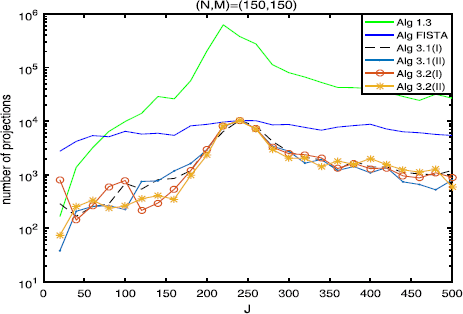
    Numbers of projections with \(\pmb{(N,M)=(150,150)}\) .

    Figure 4
    figure 4

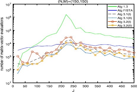
    Numbers of matrix-vector evaluations with \(\pmb{(N,M)=(150,150)}\) .

    Figure 5
    figure 5

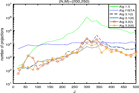
    Numbers of projections with \(\pmb{(N,M)=(200,250)}\) .

    Figure 6
    figure 6

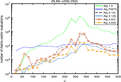
    Numbers of matrix-vector evaluations with \(\pmb{(N,M)=(200,250)}\) .

  4. (4)

    In Tables 1, 2 and 3, Algorithm 3.1(II) (or Algorithm 3.2(II)) has better performance than Algorithm 3.1(I) (or Algorithm 3.2(I)), maybe because the projections onto C and Q are very simple.

  5. (5)

    From Figures 1-5, it is observed that there exist peak values for Algorithms 1.3, 3.1 and 3.2, while FISTA has no peak values and is better than Algorithms 1.3, 3.1 and 3.2 near the peak values for some cases. However, for the other values of M, N, J, Algorithms 3.1 and 3.2 behave better than FISTA.

6 Conclusion

In this article we introduce two simultaneous projection algorithms and two semi-alternating projection algorithms to solve the SEP. We present larger stepsizes in (31) and (59) than those in Algorithms 2.1 and 2.2 in [15], which leads to a better contraction property and faster convergence speed of Algorithms 3.1 and 3.2. The weak convergence for the proposed methods is proved under standard conditions.

A numerical experiment is provided to illustrate that, except for FISTA, Algorithms 1.3, 3.1 and 3.2 have peak values. It is thus natural to combine our methods with inertial effects. This is one of our future research topics.

References

  1. Moudafi, A: Alternating CQ-algorithm for convex feasibility and split fixed-point problem. J. Nonlinear Convex Anal. 15(4), 809-818 (2014)

    MathSciNet  MATH  Google Scholar 

  2. Attouch, H, Cabot, H, Frankel, F, Peypouquet, J: Alternating proximal algorithms for constrained variational inequalities: application to domain decomposition for PDE’s. Nonlinear Anal. 74(18), 7455-7473 (2011)

    Article  MathSciNet  MATH  Google Scholar 

  3. Attouch, H, Bolte, J, Redont, P, Soubeyran, A: Alternating proximal algorithms for weakly coupled minimization problems: applications to dynamical games and PDEs. J. Convex Anal. 15, 485-506 (2008)

    MathSciNet  MATH  Google Scholar 

  4. Censor, Y, Bortfeld, T, Martin, B, Trofimov, A: A unified approach for inversion problems in intensity-modulated radiation therapy. Phys. Med. Biol. 51, 2353-2365 (2006)

    Article  Google Scholar 

  5. Attouch, H: Alternating minimization and projection algorithms. From convexity to nonconvexity. Communication in Instituto Nazionale di Alta Matematica Citta Universitaria - Roma, Italy, 8-12 June (2009)

  6. Moudafi, A: A relaxed alternating CQ-algorithm for convex feasibility problems. Nonlinear Anal. 79, 117-121 (2013)

    Article  MathSciNet  MATH  Google Scholar 

  7. Tian, D, Shi, L, Chen, R: Iterative algorithm for solving the multiple-sets split equality problem with split self-adaptive step size in Hilbert spaces. J. Inequal. Appl. 2016, 34 (2016)

    Article  MathSciNet  MATH  Google Scholar 

  8. Dong, QL, He, SN: Modified projection algorithms for solving the split equality problems. Sci. World J. 2014, 328787 (2014)

    Google Scholar 

  9. Dong, QL, He, SN: Self-adaptive projection algorithms for solving the split equality problems. Fixed Point Theory 18(1), 191-202 (2017)

    Article  MathSciNet  MATH  Google Scholar 

  10. Masad, E, Reich, S: A note on the multiple-set split convex feasibility problem in Hilbert space. J. Nonlinear Convex Anal. 8, 367-371 (2007)

    MathSciNet  MATH  Google Scholar 

  11. Byrne, C, Censor, Y, Gibali, A, Reich, S: The split common null point problem. J. Nonlinear Convex Anal. 13, 759-775 (2012)

    MathSciNet  MATH  Google Scholar 

  12. Byrne, C, Moudafi, A: Extensions of the CQ algorithm for the split feasibility and split equality problems. Working paper UAG (2013)

  13. Moudafi, A, Al-Shemas, E: Simultaneous iterative methods for split equality problems and applications. Trans. Math. Program. Appl. 1, 1-11 (2013)

    Google Scholar 

  14. Korpelevich, GM: The extragradient method for finding saddle points and other problems. Èkon. Mat. Metody 12, 747-756 (1976)

    MathSciNet  MATH  Google Scholar 

  15. Chuang, CS, Du, WS: Hybrid simultaneous algorithms for the split equality problem with applications. J. Inequal. Appl. 2016, 198 (2016)

    Article  MathSciNet  MATH  Google Scholar 

  16. Tseng, P: A modified forward–backward splitting method for maximal monotone mappings. SIAM J. Control Optim. 38, 431-446 (2000)

    Article  MathSciNet  MATH  Google Scholar 

  17. Dong, QL, He, SN, Zhao, J: Solving the split equality problem without prior knowledge of operator norms. Optimization 64(9), 1887-1906 (2015)

    Article  MathSciNet  MATH  Google Scholar 

  18. Polyak, BT: Some methods of speeding up the convergence of iteration methods. USSR Comput. Math. Math. Phys. 4, 1-17 (1964)

    Article  Google Scholar 

  19. Polyak, BT: Introduction to Optimization. Optimization Software Inc., Publications Division, New York (1987)

    MATH  Google Scholar 

  20. Dong, QL, Jiang, D: Solve the split equality problem by a projection algorithm with inertial effects. J. Nonlinear Sci. Appl. 10, 1244-1251 (2017)

    Article  MathSciNet  Google Scholar 

  21. Beck, A, Teboulle, M: A fast iterative shrinkage-thresholding algorithm for linear inverse problems. SIAM J. Imaging Sci. 2(1), 183-202 (2009)

    Article  MathSciNet  MATH  Google Scholar 

  22. Chambolle, A, Dossal, C: On the convergence of the iterates of the “Fast iterative shrinkage/thresholding algorithm”. J. Optim. Theory Appl. 166, 968-982 (2015)

    Article  MathSciNet  MATH  Google Scholar 

  23. Zhao, J: Solving split equality fixed-point problem of quasi-nonexpansive mappings without prior knowledge of operators norms. Optimization 64(12), 2619-2630 (2015)

    Article  MathSciNet  MATH  Google Scholar 

  24. Cai, X, Gu, G, He, B: On the \(O(1/t)\) convergence rate of the projection and contraction methods for variational inequalities with Lipschitz continuous monotone operators. Comput. Optim. Appl. 57, 339-363 (2014)

    Article  MathSciNet  MATH  Google Scholar 

  25. Goebel, K, Reich, S: Uniform Convexity, Hyperbolic Geometry, and Nonexpansive Mappings. Dekker, New York (1984)

    MATH  Google Scholar 

  26. Bauschke, HH, Combettes, PL: Convex Analysis and Monotone Operator Theory in Hilbert Spaces. Springer, Berlin (2011)

    Book  MATH  Google Scholar 

  27. Rockafellar, RT: Monotone operators and the proximal point algorithm. SIAM J. Control Optim. 14(5), 877-898 (1976)

    Article  MathSciNet  MATH  Google Scholar 

  28. Cegielski, A: Iterative Methods for Fixed Point Problems in Hilbert Spaces. Lecture Notes in Mathematics. Springer, Berlin (2013)

    Book  MATH  Google Scholar 

  29. Censor, Y, Elfving, T: A multiprojection algorithm using Bregman projections in a product space. Numer. Algorithms 8, 221-239 (1994)

    Article  MathSciNet  MATH  Google Scholar 

  30. Censor, Y, Bortfeld, T, Martin, B, Trofimov, A: A unified approach for inversion problems in intensity modulated radiation therapy. Phys. Med. Biol. 51, 2353-2365 (2006)

    Article  Google Scholar 

  31. Cegielski, A, Gibali, A, Reich, S: An algorithm for solving the variational inequality problem over the fixed point set of a quasi-nonexpansive operator in Euclidean space. Numer. Funct. Anal. Optim. 34, 1067-1096 (2013)

    Article  MathSciNet  MATH  Google Scholar 

  32. Reich, S, Zalas, R: A modular string averaging procedure for solving the common fixed point problem for quasi-nonexpansive mappings in Hilbert space. Numer. Algorithms 72(2), 297-323 (2016)

    Article  MathSciNet  MATH  Google Scholar 

  33. Aleyner, A, Reich, S: Block-iterative algorithms for solving convex feasibility problems in Hilbert and in Banach spaces. J. Math. Anal. Appl. 343(1), 427-435 (2008)

    Article  MathSciNet  MATH  Google Scholar 

  34. Gibali, A: A new split inverse problem and application to least intensity feasible solutions. Pure Appl. Funct. Anal. 2(2), 243-258 (2017)

    MathSciNet  MATH  Google Scholar 

  35. Censor, Y, Gibali, A, Reich, S: Algorithms for the split variational inequality problem. Numer. Algorithms 59, 301-323 (2012)

    Article  MathSciNet  MATH  Google Scholar 

Download references

Acknowledgements

The authors are supported by the National Natural Science Foundation of China (No. 71602144) and Open Fund of Tianjin Key Lab for Advanced Signal Processing (No. 2016ASP-TJ01). The authors would like to thank two anonymous referees for their careful reading of an earlier version of this paper and constructive suggestions. In particular, one referee gave us very valuable comments on the numerical experiments, and we added Section 3.2 under his opinions, which enabled us to improve the paper greatly.

Author information

Authors and Affiliations

Authors

Contributions

All authors contributed equally to the writing of this paper. All authors read and approved the final manuscript.

Corresponding author

Correspondence to Qiao-Li Dong.

Ethics declarations

Competing interests

The authors declare that they have no competing interests.

Additional information

Publisher’s Note

Springer Nature remains neutral with regard to jurisdictional claims in published maps and institutional affiliations.

Rights and permissions

Open Access This article is distributed under the terms of the Creative Commons Attribution 4.0 International License (http://creativecommons.org/licenses/by/4.0/), which permits unrestricted use, distribution, and reproduction in any medium, provided you give appropriate credit to the original author(s) and the source, provide a link to the Creative Commons license, and indicate if changes were made.

Reprints and permissions

About this article

Check for updates. Verify currency and authenticity via CrossMark

Cite this article

Dong, QL., Jiang, D. Simultaneous and semi-alternating projection algorithms for solving split equality problems. J Inequal Appl 2018, 4 (2018). https://doi.org/10.1186/s13660-017-1595-5

Download citation

  • Received:

  • Accepted:

  • Published:

  • DOI: https://doi.org/10.1186/s13660-017-1595-5

MSC

Keywords