Regularity of Parabolic Hemivariational Inequalities with Boundary Conditions

Abstract

We prove the regularity for solutions of parabolic hemivariational inequalities of dynamic elasticity in the strong sense and investigate the continuity of the solution mapping from initial data and forcing term to trajectories.

1. Introduction

In this paper, we deal with the existence and a variational of constant formula for solutions of a parabolic hemivariational inequality of the form:

(1.1)

(1.2)

(1.3)

(1.4)

(1.5)

where is a bounded domain in with sufficiently smooth boundary Let , , The boundary is composed of two pieces and , which are nonempty sets and defined by

(1.6)

where is the unit outward normal vector to . Here , is the displacement, is the strain tensor, , is a multi-valued mapping by filling in jumps of a locally bounded function , . A continuous map from the space of symmetric matrices into itself is defined by

(1.7)

where is the identity of , denotes the trace of , and , . For example, in the case , , where is Young's modulus, is Poisson's ratio and is the density of the plate.

Let and be two complex Hilbert spaces. Assume that is a dense subspace in and the injection of into is continuous. Let be a continuous linear operator from into which is assumed to satisfy Gårding's inequality. Namely, we formulated the problem (1.1) as

(1.8)

The existence of global weak solutions for a class of hemivariational inequalities has been studied by many authors, for example, parabolic type problems in [1–4], and hyperbolic types in [5–7]. Rauch [8] and Miettinen and Panagiotopoulos [1, 2] proved the existence of weak solutions for elliptic one. The background of these variational problems are physics, especially in solid mechanics, where nonconvex and multi-valued constitutive laws lead to differential inclusions. We refer to [3, 4] to see the applications of differential inclusions. Most of them considered the existence of weak solutions for differential inclusions of various forms by using the Faedo-Galerkin approximation method.

In this paper, we prove the existence and a variational of constant formula for strong solutions of parabolic hemivariational inequalities. The plan of this paper is as follows. In Section 2, the main results besides notations and assumptions are stated. In order to prove the solvability of the linear case with we establish necessary estimates applying the result of Di Blasio et al. [9] to (1.1)–(1.5) considered as an equation in as well as . The existence and regularity for the nondegenerate nonlinear systems has been developed as seen in [10, Theorem 4.1] or [11, Theorem 2.6], and the references therein. In Section 3, we will obtain the existence for solutions of (1.1)–(1.5) by converting the problem into the contraction mapping principle and the norm estimate of a solution of the above nonlinear equation on . Consequently, if is a solution asociated with , and , in view of the monotonicity of , we show that the mapping

(1.9)

is continuous.

2. Preliminaries and Linear Hemivariational Inequalities

We denote for , and for . Throughout this paper, we consider

(2.1)

We denote the dual space of , the dual pairing between and .

The norms on , , and will be denoted by , and , respectively. For the sake of simplicity, we may consider

(2.2)

We denote by . Let be the operator associated with a sesquilinear form which is defined Gårding's inequality

(2.3)

that is,

(2.4)

Then is a symmetric bounded linear operator from into which satisfies

(2.5)

and its realization in which is the restriction of to

(2.6)

is also denoted by . Here, we note that is dense in . Hence, it is also dense in . We endow the domain of with graph norm, that is, for , we define . So, for the brevity, we may regard that for all . It is known that— generates an analytic semigroup in both and .

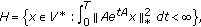
From the following inequalities

(2.7)

it follows that there exists a constant such that

(2.8)

So, we may regard as where is the real interpolation space between and .

Consider the following initial value problem for the abstract linear parabolic type equation:

(LE)

A continuous map from the space of symmetric matrices into itself is defined by

(2.9)

It is easily known that

(2.10)

(2.11)

Note that the map is linear and symmetric and it can be easily verified that the tensor satisfies the condition

(2.12)

Let be the smallest positive constant such that

(2.13)

Simple calculations and Korn's inequality yield that

(2.14)

and hence is equivalent to the norm on Then by virtue of [9, Theorem 3.3], we have the following result on the linear parabolic type equation (LE).

Proposition 2.1.

Suppose that the assumptions stated above are satisfied. Then the following properties hold.

(1)For any and , there exists a unique solution of (LE) belonging to

(2.15)

and satisfying

(2.16)

where is a constant depending on .

(2)Let and for any . Then there exists a unique solution of (LE) belonging to

(2.17)

and satisfying

(2.18)

where is a constant depending on .

Proof.

• (1) Let be a bounded sesquilinear form defined in by

  

  (2.19)

Noting that by(2.10)

(2.20)

and by (2.12), (2.14), and (1.6),

(2.21)

it follows that there exist and such that

(2.22)

Let be the operator associated with this sesquilinear form:

(2.23)

Then is also a symmetric continuous linear operator from into which satisfies

(2.24)

So we know that— generates an analytic semigroup in both and . Hence, by applying [9, Theorem 3.3] to the regularity for the solution of the equation:

(2.25)

in the space , we can obtain a unique solution of (LE) belonging to

(2.26)

and satisfying the norm estimate (2.16).

• (2) It is easily seen that

  

  (2.27)

for the time . Therefore, in terms of the intermediate theory we can see that

(2.28)

and follow the argument of (1) term by term to deduce the proof of (2) results.

3. Existence of Solutions in the Strong Sense

This Section is to investigate the regularity of solutions for the following parabolic hemivariational inequality of dynamic elasticity in the strong sense:

(HIE)

Now, we formulate the following assumptions.

(Hb) Let be a locally bounded function verifying

(3.1)

where We denote

(3.2)

The multi-valued function is obtained by filling in jumps of a function by means of the functions as follows.

(3.3)

We denote , for . We will need a regularization of defined by

(3.4)

where and It is easy to show that is continuous for all and satisfy the same condition (Hb) with possibly different constants if satisfies (Hb). It is also known that is locally Lipschitz continuous in , that is for any , there exists a number such that

(Hb-1)

(3.5)

holds for all with We denote

(3.6)

The following lemma is from [[12]; Lemma A.5].

Lemma 3.1.

Let satisfying for all and be a constant. Let be a continuous function on satisfying the following inequality:

(3.7)

Then,

(3.8)

Proof.

Let

(3.9)

Then

(3.10)

and

(3.11)

Hence, we have

(3.12)

Since is absolutely continuous and

(3.13)

for all , it holds

(3.14)

that is,

(3.15)

Therefore, combining this with (3.11), we conclude that

(3.16)

for arbitrary .

From now on, we establish the following results on the local solvability of the following equation,

(HIE-1)

Lemma 3.2.

Let be a solution of (HIE-1) and . Then, the following inequality holds, for any ,

(3.17)

where .

Proof.

We remark that from (2.11), (2.12), it follows that there is a constant such that

(3.18)

Consider the following equation:

(3.19)

Multipying on both sides of , we get

(3.20)

and integrating this over , by (1.6), (2.5), (3.18) and (Hb-1), we have

(3.21)

that is,

(3.22)

Applying Gronwall lemma, the proof of the lemma is complete.

Theorem 3.3.

Assume that , and (Hb). Then, there exists a time such that (HIE-1) admits a unique solution

(3.23)

Proof.

Assume that (2.5) holds for . Let the constant satisfy the following inequality:

(3.24)

Let us fix such that

(3.25)

where is given by (Hb).

Invoking Proposition 2.1, for a given , the problem

(HIE-2)

has a unique solution . To prove the existence and uniqueness of solutions of semilinear type (HIE-1), by virtue of Lemma 3.2, we are going to show that the mapping defined by maps is strictly contractive from into itself if the condition (3.25) is satisfied.

Lemma 3.4.

Let be the solutions of (HIE-2) with replaced by where is the ball of radius centered at zero of , respectively. Then the following inequality holds:

(3.26)

where

(3.27)

Proof.

Let be the solutions of (HIE-2) with replaced by , respectively. Then, we have that

(3.28)

Multiplying on both sides of and by (2.8), we get

(3.29)

and so, by (3.18), (2.5), (Hb), we obtain

(3.30)

Putting

(3.31)

and integrating (3.30) over , this yields

(3.32)

From (3.32) it follows that

(3.33)

Integrating (3.33) over we have

(3.34)

thus, we get

(3.35)

From (3.32) and (3.35) it follows that

(3.36)

which implies

(3.37)

By using Lemma 3.1, we obtain that

(3.38)

The proof of lemma is complete.

From (3.26) and (3.36) it follows that

(3.39)

Starting from the initial value , consider a sequence satisfying

(3.40)

Then from (3.39) it follows that

(3.41)

So by virtue of the condition (3.25) the contraction principle gives that there exists such that

(3.42)

and hence, from (3.41) there exists such that

(3.43)

Now, we give a norm estimation of the solution (HIE) and establish the global existence of solutions with the aid of norm estimations.

Theorem 3.5.

Let the assumption (Hb) be satisfied. Assume that and for any . Then, the solution of (HIE) exists and is unique in

(3.44)

Furthermore, there exists a constant depending on such that

(3.45)

Proof.

Let be the solution of

(3.46)

Then, since

(3.47)

by multiplying by , from (Hb), (3.18) and the monotonicity of , we obtain

(3.48)

By integrating on (3.48) over we have

(3.49)

By the procedure similar to (3.39) we have

(3.50)

Put

(3.51)

Then it holds

(3.52)

and hence, from (2.16) in Proposition 2.1, we have that

(3.53)

for some positive constant . Noting that by (Hb)

(3.54)

and by Proposition 2.1

(3.55)

it is easy to obtain the norm estimate of in satisfying (3.45).

Now from Theorem 3.3 it follows that

(3.56)

So, we can solve the equation in and obtain an analogous estimate to (3.53). Since the condition (3.25) is independent of initial values, the solution of (HIE-1) can be extended the internal for a natural number , that is, for the initial in the interval , as analogous estimate (3.53) holds for the solution in . Furthermore, the estimate (3.45) is easily obtained from (3.53) and (3.56).

We show that is a solution of the problem (HIE). Lemma 3.4 and (Hb) give that

(3.57)

and for , there exists a unique solution of (HIE) belonging to

(3.58)

and satisfying (3.44).

From (3.44)and (3.57), we can extract a subsequence from , still denoted by , such that

(3.59)

(3.60)

Here, we remark that if is compactly embedded in and , the following embedding

(3.61)

is compact in view [13, Theorem 2]. Hence, the mapping

(3.62)

By a solution of (HIE-1), we understand a mild solution that has a form

(3.63)

so letting and using the convergence results above, we obtain

(3.64)

Now, we show that a.e. in . Indeed, from (3.62) we have strongly in and hence a.e. in for each Let and Using the theorem of Lusin and Egoroff, we can choose a subset such that and uniformly on Thus, for each there is an such that

(3.65)

Then, if we have for all and

Therefore we have

(3.66)

Let Then

(3.67)

Letting in this inequality and using (3.60), we obtain

(3.68)

where Letting in this inequality, we deduce that

(3.69)

and letting we get

(3.70)

This implies that a.e. in This completes the proof of theorem.

Remark 3.6.

In terms of Proposition 2.1, we remark that if and for any then the solution of (HIE) exists and is unique in

(3.71)

Futhermore, there exists a constant depending on such that

(3.72)

Theorem 3.7.

Let the assumption (Hb) be satisfied

(1)if , then the solution of (HIE) belongs to and the mapping

(3.73)

is continuous.

• (2) let . Then the solution of (HIE) belongs to and the mapping

  

  (3.74)

is continuous.

Proof.

• (1) It is easy to show that if and , then belongs to . let and be the solution of (HIE) with in place of for Then in view of Proposition 2.1, we have

  

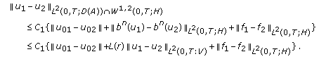  (3.75)

Since

(3.76)

we get

(3.77)

Hence, arguing as in (2.8), we get

(3.78)

Combining (3.75) with (3.78), we obtain

(3.79)

Suppose that in and let and be the solutions (HIE) with and , respectively. Let be such that

(3.80)

Then by virtue of (3.79) with replaced by we see that

(3.81)

This implies that in . Hence the same argument shows that in

(3.82)

Repeating this process we conclude that in

• (2) If then belongs to from Theorem 3.5. Let and be the solution of (HIE) with in place of for . Multiplying (HIE) by , we have

  

  (3.83)

Put

(3.84)

Then, by the similar argument in (3.32), we get

(3.85)

and we have that

(3.86)

thus, arguing as in (3.35) we have

(3.87)

Combining this inequality with (3.85) it holds that

(3.88)

By Lemma 3.1 the following inequality

(3.89)

implies that

(3.90)

Hence, from (3.88) and (3.90) it follows that

(3.91)

The last term of (3.91) is estimated as

(3.92)

Let be such that

(3.93)

Hence, from (3.91) and (3.92) it follows that there exists a constant such that

(3.94)

Suppose in , and let and be the solutions (HIE) with and , respectively. Then, by virtue of (3.94), we see that in . This implies that in . Therefore the same argument shows that in

(3.95)

Repeating this process, we conclude that in .

References

Miettinen M: A parabolic hemivariational inequality. Nonlinear Analysis: Theory, Methods & Applications 1996,26(4):725–734. 10.1016/0362-546X(94)00312-6
Miettinen M, Panagiotopoulos PD: On parabolic hemivariational inequalities and applications. Nonlinear Analysis: Theory, Methods & Applications 1999,35(7):885–915. 10.1016/S0362-546X(97)00720-7
Panagiotopoulos PD: Inequality Problems in Mechanics and Applications: Convex and Nonconvex Energy Functions. Birkhäuser, Boston, Mass, USA; 1985:xx+412.
Panagiotopoulos PD: Modelling of nonconvex nonsmooth energy problems. Dynamic hemivariational inequalities with impact effects. Journal of Computational and Applied Mathematics 1995,63(1–3):123–138.
Park JY, Kim HM, Park SH: On weak solutions for hyperbolic differential inclusion with discontinuous nonlinearities. Nonlinear Analysis: Theory, Methods & Applications 2003,55(1–2):103–113. 10.1016/S0362-546X(03)00216-5
Park JY, Park SH: On solutions for a hyperbolic system with differential inclusion and memory source term on the boundary. Nonlinear Analysis: Theory, Methods & Applications 2004,57(3):459–472. 10.1016/j.na.2004.02.024
Migórski S, Ochal A: Vanishing viscosity for hemivariational inequalities modeling dynamic problems in elasticity. Nonlinear Analysis: Theory, Methods & Applications 2007,66(8):1840–1852. 10.1016/j.na.2006.02.028
Rauch J: Discontinuous semilinear differential equations and multiple valued maps. Proceedings of the American Mathematical Society 1977,64(2):277–282. 10.1090/S0002-9939-1977-0442453-6
Di Blasio G, Kunisch K, Sinestrari E: -regularity for parabolic partial integro-differential equations with delay in the highest-order derivatives. Journal of Mathematical Analysis and Applications 1984,102(1):38–57. 10.1016/0022-247X(84)90200-2
Ahmed NU: Optimization and Identification of Systems Governed by Evolution Equations on Banach Space, Pitman Research Notes in Mathematics Series. Volume 184. Longman Scientific & Technical, Harlow, UK; 1988:vi+187.
Barbu V: Nonlinear Semigroups and Differential Equations in Banach Spaces. Nordhoff, Leiden, The Netherlands; 1976:352.
Brézis H: Opérateurs Maximaux Monotones et Semigroupes de Contractions dans un Espace de Hilbert. North Holland, Amsterdam, The Netherlands; 1973.
Aubin J-P: Un théorème de compacité. Comptes Rendus de l'Académie des Sciences 1963, 256: 5042–5044.
Acknowledgment
The authors wish to thank the referees for careful reading of manuscript, for valuable suggestions and many useful comments.
Author information
Authors and Affiliations
Corresponding author
Rights and permissions
Open Access This article is distributed under the terms of the Creative Commons Attribution 2.0 International License ( https://creativecommons.org/licenses/by/2.0 ), which permits unrestricted use, distribution, and reproduction in any medium, provided the original work is properly cited.
About this article
Cite this article
Park, DG., Jeong, JM. & Park, S.H. Regularity of Parabolic Hemivariational Inequalities with Boundary Conditions. J Inequal Appl 2009, 207873 (2009). https://doi.org/10.1155/2009/207873
Received:
Revised:
Accepted:
Published:
DOI: https://doi.org/10.1155/2009/207873
Comments
View archived comments (1)