Noise-induced transitions in an avian influenza model with the Allee effect

Abstract

This paper presents noise-induced transitions in a stochastic avian influenza model with Allee effect. In the deterministic case, one of three disease-free equilibria is always globally asymptotically stable in its attractive domain, and there is a unique endemic equilibrium when the basic reproduction number $R_{0}>1$. In the stochastic case, a new dynamic phenomenon of noise-induced transition can be observed, that is, the stochastic trajectory can exit from the neighborhood of the epidemic equilibrium and pass into the vicinity of the trivial equilibrium. More precisely, in this paper, based on the stochastic sensitivity function technique, we construct the confidence ellipse and then estimate the critical value of the noise intensity leading to extinction. We also propose useful control strategies to prevent the noise-induced extinction.

1 Introduction

Avian influenza (bird flu) refers to the disease caused by infection with avian (bird) influenza (flu) Type A viruses. These viruses naturally spread among wild aquatic birds worldwide and can infect domestic poultry and other bird and animal species [1]. Influenza A virus can be divided into H subtypes and N subtypes according to different proteins on the surface of the virus: hemagglutinin (HA) and neuraminidase (NA) [2]. It was formerly believed that avian influenza viruses are distinct from human influenza viruses and cannot spread easily to human. However, in 1997, cases of human infection with highly pathogenic avian influenza A (H5N1) virus were reported during an avian influenza outbreak in Hong Kong, China. After that, infection to human of avian influenza occurred successively. Influenza A virus has spread from Asia to Europe, Africa, and the Middle East since 2003 and resulted in millions of poultry infections, hundreds of human cases and deaths in more than 50% of human cases [3]. Another identified influenza A viruses associated with human infections are H7N9 viruses, which were first detected in China in 2013. While human infections with H7N9 viruses are uncommon, they have resulted in severe respiratory illness and death in approximately 40 of reported cases [2]. Data from the Ministry of Agriculture and Rural Affairs shows that in the first quarter of 2022, there were 1526 cases of avian influenza in the world (excluding wild birds), affecting 21 countries, and a large number of poultry were culled.

In order to prevent the endangerment of wild birds and stop avian influenza from becoming a global disease, various mathematical models have been used to analyze the epidemiological characteristics of avian influenza and propose useful control measures [4, 5]. Iwami et al. [6] constructed an avian-human influenza epidemic model to investigate relations between the evolution of virulence and an effectiveness of pandemic control measures after the emergence of mutant avian influenza: one is an elimination policy of infected birds with avian influenza and the other is a quarantine policy of infected humans with mutant avian influenza. They found that each of these prevention policies may be ineffective, and the quarantine policy can effectively reduce both human morbidity and mortality, but the elimination policy increases either human morbidity or mortality in a worst case situation. Zhang et al. [7] developed a dynamic model of resident birds and poultry. They concluded that although closing the live poultry trading market is not the main measure to control the epidemic, but it can control the epidemic to a lower level.

In particular, Liu [8] formulated a classic avian-only influenza model:

$$\begin{aligned} \textstyle\begin{cases} \frac{{\mathrm{d}}S_{a}(t)}{{\mathrm{d}}t}=g(S_{a}(t))-\beta _{a} S_{a}(t)I_{a}(t), \\ \frac{{\mathrm{d}}I_{a}(t)}{{\mathrm{d}}t}=\beta _{a} S_{a}(t)I_{a}(t)-(\mu _{a}+ \delta _{a})I_{a}(t), \end{cases}\displaystyle \end{aligned}$$

(1.1)

where $S_{a}(t)$ and $I_{a}(t)$ represent the susceptible and the infective at time t, respectively, $\beta _{a}$ is the transmission rate from infective avian to susceptible avian, $\mu _{a}$ is the natural death rate of the avian population, $\delta _{a}$ is the disease-related death rate of infected avian. It is well known that the population growth rate is related to both population size and available resources, so the logistic growth is more realistic than the constant growth for the wildlife birds, then $g(S_{a})=r_{a}S_{a}(1-\frac{S_{a}}{K_{a}})$, where $r_{a}$ is the intrinsic growth rate and $K_{a}$ is the maximal carrying capacity of the avian population. As one of the main sources for transmitting disease to humans, avian populations are assumed to experience a strong Allee effect, a phenomenon in which the species will become extinct when the population density falls below a certain threshold due to factors such as difficulty in finding a mate, genetic inbreeding, or a reduction in cooperative interactions [9]. In other words, strong Allee effect can lead to complex dynamics in epidemic and population models [10]. If the susceptible avian population is subject to Allee effect, then $g(S_{a})=r_{a}S_{a} (1-\frac{S_{a}}{M_{a}} ) ( \frac{S_{a}}{m_{a}}-1 )$, where $M_{a}$ is the maximal carrying capacity of the avian population and $m_{a}$ is the critical carrying capacity of the avian population.

However, populations are inevitably influenced by environmental factors such as climate, water resources, and diseases. There are different possible approaches to introduce noise into stochastic differential equations, both from a biological and from a mathematical perspective. One traditional approach is analogous to that of Beddington and May [11] who superimposed a one-dimensional white noise process into the density-independent term. In fact, stochastic models have been employed to study unexpected phenomena that do not occur in the deterministic models, such as noise-induced transitions [12, 13], noise-induced chaos [14], and noise-induced complexity [15–17]. Bashkirtseva and Ryashko [18] studied noise-induced transitions from the zone of coexistence to the zone of extinction for the stochastically forced predator–prey population model with Allee effect. Bashkirtseva et al. [19] considered a phenomenological Hassell mathematical model with Allee effect and found that the persistence zone can decrease and even disappear under the influence of random noise. Yuan et al. [20] considered a stochastically forced producer-grazer model and studied the phenomenon of noise-induced state switching between two stochastic attractors in the bistable zone. They constructed the confidence ellipse and the confidence band to find the configurational arrangement of equilibria and a limit cycle, respectively. Moreover, Ruan [21] introduced a semi-analytical method to explore the asymptotically convergent behavior of a stochastic avian model with Allee effect and explored that an increased noise could lead to stability transition from bistability to monostability.

Based on the above discussions, we attempt to study the phenomena of noise-induced transitions for avian influenza model with Allee effect by using the stochastic sensitivity function technique. The paper is organized as follows. In Sect. 2, we review the deterministic avian influenza model and establish its stochastic version. The analysis and control of the noise-induced extinction will be presented in Sect. 3. We finally conclude the paper by some discussions in Sect. 4. Some mathematical background of the stochastic sensitivity function technique will be briefly outlined in the Appendix.

2 Model formulation

2.1 Deterministic avian influenza model with the Allee effect

To study the influence of noise perturbation on the dynamic behaviors, we recall the well-defined model (1.1) with the Allee effect and obtain the following deterministic model:

$$\begin{aligned} \textstyle\begin{cases} \frac{{\mathrm{d}}S_{a}(t)}{{\mathrm{d}}t}=r_{a}S_{a}(t) (1- \frac{S_{a}(t)}{M_{a}} ) (\frac{S_{a}(t)}{m_{a}}-1 )- \beta _{a} S_{a}(t)I_{a}(t), \\ \frac{{\mathrm{d}}I_{a}(t)}{{\mathrm{d}}t}=\beta _{a} S_{a}(t)I_{a}(t)-(\mu _{a}+ \delta _{a})I_{a}(t). \end{cases}\displaystyle \end{aligned}$$

(2.1)

Define the basic reproduction number by

$$\begin{aligned} \mathcal{R}_{0}= \frac{\beta _{a}(M_{a}+m_{a})(\mu _{a}+\delta _{a})}{(\mu _{a}+\delta _{a})^{2}+M_{a}m_{a}\beta _{a}^{2}}. \end{aligned}$$

According to [8, Theorem 3.5], system (2.1) has the following dynamic properties:

• System (2.1) always has three disease-free equilibria given by $E_{0}=(0,0)$, $E_{1}=(m_{a},0)$, $E_{2}=(M_{a},0)$; if $\mathcal{R}_{0}>1$ or, equivalently, $m_{a}<\frac{\mu _{a}+\delta _{a}}{\beta _{a}}<M_{a}$, system (2.1) also has a unique endemic equilibrium $E_{3}=(S_{a}^{*},I_{a}^{*})$, where

  $$\begin{aligned} S_{a}^{*}=\frac{\mu _{a}+\delta _{a}}{\beta _{a}}, \qquad I_{a}^{*}= \frac{r_{a}}{\beta _{a}} \frac{(\mu _{a}+\delta _{a})^{2}+M_{a}m_{a}\beta _{a}^{2}}{M_{a}m_{a}\beta _{a}^{2}}( \mathcal{R}_{0}-1). \end{aligned}$$

• The disease-free equilibrium $E_{0}$ of the avian system (2.1) is always globally asymptotically stable in $D_{1}$, but the disease-free equilibrium $E_{1}$ is always unstable. If $m_{a}<\frac{\mu _{a}+\delta _{a}}{\beta _{a}}<\frac{m_{a}+M_{a}}{2}$, then system (2.1) has a unique limit cycle in the neighborhood of the endemic equilibrium $E_{3}$, which is globally asymptotically stable in $D_{2}$; if $\frac{m_{a}+M_{a}}{2}<\frac{\mu _{a}+\delta _{a}}{\beta _{a}}<M_{a}$, then the endemic equilibrium $E_{3}$ is globally asymptotically stable in $D_{2}$; if $\frac{\mu _{a}+\delta _{a}}{\beta _{a}}>M_{a}$, then the disease-free equilibrium $E_{2}$ is globally asymptotically stable in $D_{2}$.

Remark 2.1

The authors in [8] divide $\mathbb{R}_{+}^{2}$ into two subregions $D_{1}$ and $D_{2}$. Here, the vector field of system (2.1) for the case $\frac{m_{a}+M_{a}}{2}<\frac{\mu _{a}+\delta _{a}}{\beta _{a}}<M_{a}$ is shown in Fig. 1, in which the dashed-dotted line is the separatrix of two domains. For a detailed explanation of $D_{1}$ and $D_{2}$ above, please refer to Sect. 3.2.2 of Ref. [8].

Figure 1

Vector field of deterministic model (2.1) and the separatrix of two attraction domains

In order to reflect the above results intuitively, we further take the following realistic parameter values from [8] for some numerical simulations. The disease-induced death rate of the infected avian is $\delta _{a}=4\times 10^{-4}$ per day. The natural death rate $\mu _{a}$ is about $\mu _{a}=3\times 10^{-3}$ per day under the assumption that the wild avian can survive eight years. The intrinsic growth rate of the avian population is $r_{a}=5\times 10^{-4}$ per day. The transition rate from infected avian population to susceptible avian is $\beta _{a}=1\times 10^{-6}$ and the critical carrying capacity of the avian population is $m_{a}=800$. The maximal carrying capacity of the avian population $M_{a}$ is regarded as a variable parameter.

• (i) Set $M_{a}=5000$, then $\frac{m_{a}+M_{a}}{2}=2900<\frac{\mu _{a}+\delta _{a}}{\beta _{a}}=3400<M_{a}=5000$, system (2.1) has two stable states $E_{0}=(0,0)$ and $E_{3}=(3400,5200)$ (see Fig. 2(a));

  Figure 2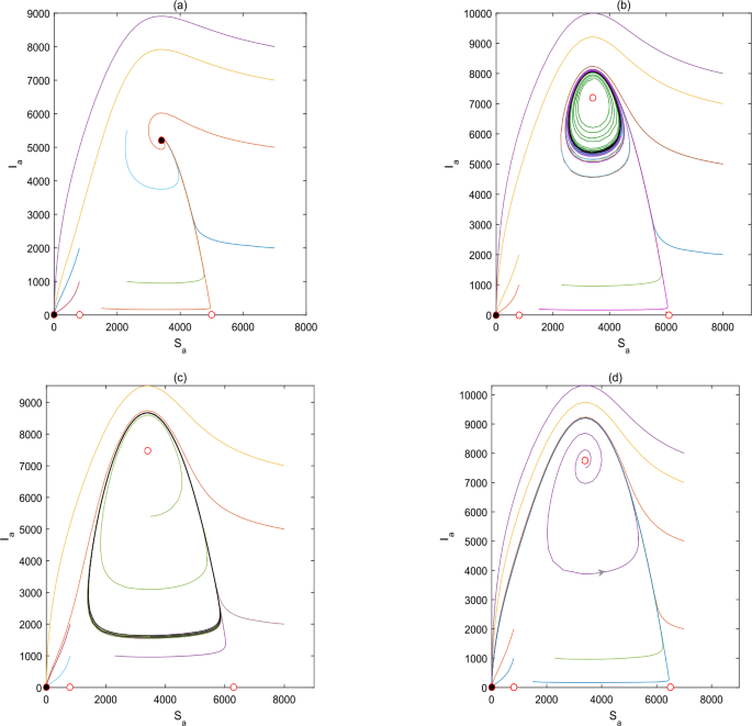

  

  The plots are the global phase portraits of the avian system (2.1) with respect to $\frac{\mu _{a}+\delta _{a}}{\beta _{a}}$. (a) $M_{a}=5000$; (b) $M_{a}=6100$; (c) $M_{a}=6300$; (d) $M_{a}=6500$

• (ii) For $M_{a}=6100$, then $m_{a}=800<\frac{\mu _{a}+\delta _{a}}{\beta _{a}}=3400< \frac{m_{a}+M_{a}}{2}=3450$, system (2.1) has two stable states $E_{0}=(0,0)$ and the limit cycle (see Fig. 2(b)). Besides, as $M_{a}$ increases, the limit cycle becomes larger (see Fig. 2(c)).

• (iii) As $M_{a}$ increases to 6500, then $m_{a}=800<\frac{\mu _{a}+\delta _{a}}{\beta _{a}}=3400< \frac{m_{a}+M_{a}}{2}=3650$, the limit cycle disappears and there exists only one stable state $E_{0}=(0,0)$ for system (2.1) (see Fig. 2(d)).

2.2 Stochastic avian influenza model with the Allee effect

In this subsection, we introduce multiplicative noises into deterministic model (2.1) by perturbing the growth rate $r_{a}$ and the death rate $\delta _{a}$ by $r_{a}+\sigma \dot{B}_{1}(t)$ and $\delta _{a}+\sigma \dot{B}_{2}(t)$, respectively, obtaining the stochastic avian influenza model with Allee effect:

$$\begin{aligned} \textstyle\begin{cases} {\mathrm{d}}S_{a}(t)=S_{a}(t) (1-\frac{S_{a}(t)}{M_{a}} ) (\frac{S_{a}(t)}{m_{a}}-1 )(r_{a}{\,\mathrm{d}}t+\sigma{\,\mathrm{d}}B_{1}(t)){ \,\mathrm{d}}t-\beta S_{a}(t)I_{a}(t){\,\mathrm{d}}t, \\ {\mathrm{d}}I_{a}(t)=(\beta S_{a}(t)I_{a}(t)-(\mu _{a}+\delta _{a})I_{a}(t)){ \,\mathrm{d}}t+\sigma I_{a}(t){\,\mathrm{d}}B_{2}(t), \end{cases}\displaystyle \end{aligned}$$

(2.2)

where $B_{i}(t)$, $i=1,2$, are mutually independent Brown motions and σ is the noise intensity.

We start with a basic theorem about the well-posedness of the model.

Theorem 2.1

For any given initial value $(S_{a}(0), I_{a}(0))\in \mathbb{R}_{+}^{2}$, system (2.2) has a unique global solution $(S_{a}(t), I_{a}(t))$ on $t \geq 0$, and the solution will always remain in $\mathbb{R}_{+}^{2}$ with probability 1.

Proof

The drift and the diffusion of system (2.2) are locally Lipschitz continuous, for any initial value $(S_{a}(0),I_{a}(0))\in \mathbb{R}^{2}_{+}$, there is a unique local solution $(S_{a}(t),I_{a}(t))\in [0,\tau _{e})$, where $\tau _{e}$ is the explosion time. To show the solution is global, we only need to verify that $\tau _{e}=\infty$ a.s. Let $k_{0}>0$ be sufficiently large so that $(S_{a}(0),I_{a}(0))$ lies within the interval $[\frac{1}{k_{0}},k_{0}]\times [\frac{1}{k_{0}},k_{0}]$. For each $k>k_{0}$, define the stoping time

$$\begin{aligned} \tau _{k}=\inf \biggl\{ t\in [0,\tau _{e}):\min \bigl\{ S_{a}(t),I_{a}(t)\bigr\} \leq \frac{1}{k} \ \mathrm{or}\ \max \bigl\{ S_{a}(t),I_{a}(t)\bigr\} \geq k \biggr\} . \end{aligned}$$

Throughout this paper, we set $\inf \emptyset =+\infty$. Clearly, $\tau _{k}$ is increasing as $k\rightarrow \infty$. Set $\tau _{\infty}=\lim_{k\rightarrow \infty}\tau _{k}$, whence $\tau _{\infty}\leq \tau _{e}$ a.s. If we can prove that $\tau _{\infty}=\infty$ a.s., then $\tau _{e}=\infty$ a.s. and $(S(t),I(t))\in \mathbb{R}_{+}^{2}$ a.s. for all $t>0$ a.s. Otherwise, there are two constants $T>0$ and $\delta \in (0,1)$ such that

$$\begin{aligned} P\{\tau _{\infty}\leq T\}>\delta. \end{aligned}$$

Hence there is an integer $k_{1}\geq k_{0}$ such that for all $k\geq k_{1}$

$$\begin{aligned} P\{\tau _{k}\leq T\}\geq \delta. \end{aligned}$$

Define a nonnegative $C^{2}$-function $V: \mathbb{R}_{+}^{2}\rightarrow \mathbb{R}_{+}$ by

$$\begin{aligned} V(S_{a},I_{a})=S_{a}-l-l\ln S_{a}+l \ln l+I_{a}-1-\ln I_{a}+ \frac{1}{v}S_{a}^{v}, \end{aligned}$$

where $l=\frac{\mu _{a}+\delta _{a}}{\beta _{a}}$, v is the normal number that satisfies $0< v<1$. By using Itô’s formula, we have

$$\begin{aligned} \mathcal{L}V ={}& \biggl(1-\frac{l}{S_{a}} \biggr) \biggl(r_{a}S_{a} \biggl(1-\frac{S_{a}}{M_{a}} \biggr) \biggl(\frac{S_{a}}{m_{a}}-1 \biggr)-\beta _{a} S_{a}I_{a} \biggr) +\frac{\sigma ^{2}}{2}l \biggl(1- \frac{S_{a}}{M_{a}} \biggr)^{2} \biggl(\frac{S_{a}}{m_{a}}-1 \biggr)^{2} \\ & {}+ \biggl(1-\frac{1}{I_{a}} \biggr) \bigl(\beta _{a} S_{a}I_{a}-(\mu _{a}+ \delta _{a})I_{a}\bigr)+\frac{1}{2}\sigma ^{2}+S_{a}^{v} \biggl(r_{a} \biggl(1- \frac{S_{a}}{M_{a}} \biggr) \biggl(\frac{S_{a}}{m_{a}}-1 \biggr)- \beta _{a} I_{a} \biggr) \\ &{}-\frac{1}{2}\sigma ^{2}(1-v)S_{a}^{v} \biggl(1-\frac{S_{a}}{M_{a}} \biggr)^{2} \biggl(\frac{S_{a}}{m_{a}}-1 \biggr)^{2} \\ \leq{}& {-}\frac{\sigma ^{2}}{2M_{a}^{2}m_{a}^{2}}(1-v)S_{a}^{4+v}+ \frac{\sigma ^{2}}{2M_{a}^{2}m_{a}^{2}}S_{a}^{4} + \frac{\sigma ^{2}}{M_{a}m_{a}} \biggl( \frac{1}{M_{a}}+\frac{1}{m_{a}} \biggr) (1-v)S_{a}^{3+v} \\ &{}- \biggl(\frac{\sigma ^{2}}{M_{a}m_{a}} \biggl(\frac{1}{M_{a}}+ \frac{1}{m_{a}} \biggr)+\frac{r_{a}}{M_{a}m_{a}} \biggr)S_{a}^{3} - \frac{\sigma ^{2}}{2} \biggl(\frac{1}{M_{a}^{2}}+\frac{1}{m_{a}^{2}}+ \frac{4}{M_{a}m_{a}} \biggr) (1-v)S_{a}^{2+v} \\ &{}+ \biggl((r_{a}+r_{a}l) \biggl(\frac{1}{M_{a}}+ \frac{1}{m_{a}} \biggr)+ \frac{\sigma ^{2}}{2} \biggl(\frac{1}{M_{a}^{2}} + \frac{1}{m_{a}^{2}}+ \frac{4}{M_{a}m_{a}} \biggr) \biggr)S_{a}^{2} \\ &{}+ \biggl(\frac{1}{M_{a}}+\frac{1}{m_{a}} \biggr) \bigl(r_{a}+ \sigma ^{2}(1-v)\bigr)S_{a}^{1+v} - \biggl(r_{a}+r_{a}l+\beta _{a}+\sigma ^{2} \biggl(\frac{1}{M_{a}}+ \frac{1}{m_{a}} \biggr) \biggr)S_{a} \\ &{}+r_{a}l+\mu _{a}+\delta _{a}+ \frac{\sigma ^{2}}{2} \\ \leq{}& M. \end{aligned}$$

Following the proof of the remainder of Theorem in [22, Theorem 2.1], we obtain that system (2.2) admits a unique positive solution $(S_{a}(t), I_{a}(t))\in \mathbb{R}_{+}^{2}$ for any given initial value $(S_{a}(0), I_{a}(0))\in \mathbb{R}_{+}^{2}$. □

3 Analysis of the noise-induced transition and control system

3.1 Analysis of the noise-induced transition

Due to the complexity of system (2.2), it is not easy to obtain the analytic formula for the threshold value of noise intensity determining avian influenza population permanence and extinction. Under this circumstance, we take endemic equilibrium $E_{3}$ and the limit cycle as examples to numerically illustrate the impact of environment noise on the dynamics of model (2.2).

We screen 50 pairs of initial values by even distribution with $S_{a}$ between 0 and 7000 and $I_{a}$ between 0 and 6000, respectively. Parameters $\gamma _{a}, \delta _{a}, \mu _{a}, \beta _{a}$, and $m_{a}$ are chosen as before. Set $M_{a}=5000$, then $\frac{m_{a}+M_{a}}{2}<\frac{\mu _{a}+\delta _{a}}{\beta _{a}}<M_{a}$, i.e., deterministic model (2.1) has two stable states, disease-free equilibrium $E_{0}=(0,0)$ and endemic equilibrium $E_{3}=(3400,5200)$ (see Fig. 3(a)–(b)). For a weak noise $\sigma =1\times 10^{-3}$, the solution curves of stochastic model (2.2) starting from the attraction domain $D_{2}$ will oscillate around the endemic equilibrium $E_{3}$ (see Fig. 3(c)–(d)). As the noise intensity increases to $\sigma =1\times 10^{-2}$, the trajectories of model (2.2) will escape from the neighborhood of $E_{3}$ into domain $D_{1}$, and eventually tend to $E_{0}$ (see Fig. 3(e)–(f)).

Figure 3

(a) and (b) Times series for deterministic model (2.1); (c) and (d) Time series for stochastic model (2.2) with $\sigma =1\times 10^{-3}$; (e) and (f) Time series for stochastic model (2.2) with $\sigma =1\times 10^{-2}$

Take $M_{a}=6100$ and initial value $(S_{a}(0),I_{a}(0))=(3400,5460)$, then for fixed parameters $\gamma _{a}, \delta _{a}, \mu _{a}, \beta _{a}$, and $m_{a}$, $m_{a}<\frac{\mu _{a}+\delta _{a}}{\beta _{a}}<\frac{m_{a}+M_{a}}{2}$, i.e., system (2.1) has two stable states, disease-free equilibria $E_{0}=(0,0)$ and a limit cycle around $E_{3}$. For a weak small noise $\sigma =1\times 10^{-4}$, the stochastic cycle of system (2.2) oscillates around the deterministic limit cycle. When the noise becomes $\sigma =1\times 10^{-3}$, the trajectories of system (2.2) initially oscillate near the deterministic limit cycle, but eventually cross the separatrix and enter attraction domain $D_{1}$, tending towards $E_{0}$ (see Fig. 4).

Figure 4

(a) Time series diagrams of system (2.2) with $\sigma =1\times 10^{-4}$; (b) Deterministic cycle (solid black) and trajectories (dashed) of stochastic system (2.2); (c) Time series diagrams of system (2.2) with $\sigma =1\times 10^{-3}$; (d) Deterministic cycle (solid black) and trajectories (dashed) of stochastic system (2.2)

Figure 3 and Fig. 4 show a noise-induced transition from coexistence to extinction. For different random attractors, there exists the corresponding critical value $\sigma _{*}$ such that when $0<\sigma <\sigma _{*}$, the solution of stochastic model (2.2) oscillates around endemic equilibrium $E_{3}$ (or deterministic limit cycle), biologically, both susceptible and infected avian populations exist; when $\sigma >\sigma _{*}$, the solution of stochastic model (2.2) eventually tends to $E_{0}$, biologically, both susceptible and infected avian populations go extinct.

Consider the following boundary equation without infected avian population:

$$\begin{aligned} \mathrm{d} \widetilde{S}_{a}(t)= \widetilde{S}_{a}(t) \biggl(1- \frac{\widetilde{S}_{a}(t)}{M_{a}} \biggr) \biggl( \frac{\widetilde{S}_{a}(t)}{m_{a}}-1 \biggr) \bigl(r_{a}\,\mathrm{d} t+ \sigma \,\mathrm{d} B_{1}(t) \bigr),\quad\widetilde{S}_{a}(0)\geq 0. \end{aligned}$$

(3.1)

Lemma 3.1

If $\sigma ^{2}>\frac{4M_{a}m_{a}r_{a}}{(M_{a}-m_{a})^{2}}$, then the solution $\widetilde{S}_{a}(t)$ of system (3.1) satisfies $\lim_{t\rightarrow \infty}\widetilde{S}_{a}(t)=0$ for any $t>0$ with a probability 1.

Proof

An application of Itô’s formula leads to

$$\begin{aligned} \mathrm{d}\ln \widetilde{S}_{a}(t) ={}& \biggl[r_{a} \biggl(1- \frac{\widetilde{S}_{a}(t)}{M_{a}} \biggr) \biggl( \frac{\widetilde{S}_{a}(t)}{m_{a}}-1 \biggr) -\frac{\sigma ^{2}}{2} \biggl(1-\frac{\widetilde{S}_{a}(t)}{M_{a}} \biggr)^{2} \biggl( \frac{\widetilde{S}_{a}(t)}{m_{a}}-1 \biggr)^{2} \biggr]\, \mathrm{d}t \\ & {}+\sigma \biggl(1-\frac{\widetilde{S}_{a}(t)}{M_{a}} \biggr) \biggl( \frac{\widetilde{S}_{a}(t)}{m_{a}}-1 \biggr)\,\mathrm{d} B_{1}(t) \\ ={}& \biggl[-\frac{\sigma ^{2}}{2M_{a}^{2}m_{a}^{2}}\widetilde{S}_{a}^{4}(t)+ \frac{\sigma ^{2}}{M_{a}m_{a}} \biggl(\frac{1}{M_{a}}+\frac{1}{m_{a}} \biggr) \widetilde{S}_{a}^{3}(t) - \biggl(\frac{\sigma ^{2}}{2} \biggl( \frac{1}{M_{a}^{2}}+\frac{1}{m_{a}^{2}}+\frac{4}{M_{a}m_{a}} \biggr) \\ &{}+\frac{r_{a}}{M_{a}m_{a}} \biggr)\widetilde{S}_{a}^{2}(t)+ \bigl(r_{a}+ \sigma ^{2}\bigr) \biggl(\frac{1}{M_{a}}+ \frac{1}{m_{a}} \biggr) \widetilde{S}_{a}(t) - \biggl(r_{a}+ \frac{\sigma ^{2}}{2} \biggr) \biggr]\,\mathrm{d}t \\ &{}+\sigma \biggl(1-\frac{\widetilde{S}_{a}(t)}{M_{a}} \biggr) \biggl( \frac{\widetilde{S}_{a}(t)}{m_{a}}-1 \biggr)\,\mathrm{d} B_{1}(t). \end{aligned}$$

(3.2)

Let the function

$$\begin{aligned} f(x)={}&{-}\frac{\sigma ^{2}}{2M_{a}^{2}m_{a}^{2}}x^{4}+ \frac{\sigma ^{2}}{M_{a}m_{a}} \biggl( \frac{1}{M_{a}}+\frac{1}{m_{a}} \biggr)x^{3} \\ &{}- \biggl( \frac{\sigma ^{2}}{2} \biggl(\frac{1}{M_{a}^{2}}+ \frac{1}{m_{a}^{2}}+ \frac{4}{M_{a}m_{a}} \biggr)+ \frac{r_{a}}{M_{a}m_{a}} \biggr)x^{2} \\ &{} +\bigl(r_{a}+\sigma ^{2}\bigr) \biggl( \frac{1}{M_{a}}+\frac{1}{m_{a}} \biggr)x - \biggl(r_{a}+ \frac{\sigma ^{2}}{2} \biggr). \end{aligned}$$

Then, the derivative of $f(x)$ is

$$\begin{aligned} f'(x)=Ax^{3}+Bx^{2}+Cx+D, \end{aligned}$$

where

$$\begin{aligned} &A=-\frac{2\sigma ^{2}}{M_{a}^{2}m_{a}^{2}},\qquad B= \frac{3\sigma ^{2}}{M_{a}m_{a}} \biggl(\frac{1}{M_{a}}+ \frac{1}{m_{a}} \biggr),\\ &C=-\sigma ^{2} \biggl(\frac{1}{M_{a}^{2}}+\frac{1}{m_{a}^{2}}+ \frac{4}{M_{a}m_{a}} \biggr)-\frac{2r_{a}}{M_{a}m_{a}},\qquad D=\bigl(r_{a}+\sigma ^{2}\bigr) \biggl(\frac{1}{M_{a}}+\frac{1}{m_{a}} \biggr). \end{aligned}$$

To obtain the monotonicity of the function $f(x)$, we consider the following simple cubic equation:

$$\begin{aligned} Ax^{3}+Bx^{2}+Cx+D=0. \end{aligned}$$

(3.3)

Divide the above equation by A and let $x=y+\frac{M_{a}+m_{a}}{2}$, then (3.3) becomes

$$\begin{aligned} y^{3}+Py+Q=0, \end{aligned}$$

(3.4)

here,

$$\begin{aligned} P=-\frac{1}{4}(M_{a}-m_{a})^{2}+ \frac{r_{a}}{\sigma ^{2}}M_{a}m_{a},\qquad Q=\frac{1}{2}(M_{a}+m_{a})^{3}. \end{aligned}$$

Obviously, the discriminant $\Delta = (\frac{Q}{2} )^{2}+ (\frac{P}{3} )^{3}>0$, namely, (3.4) has a unique negative real root $y_{1}= \sqrt[3]{-\frac{Q}{2}+\sqrt{ (\frac{Q}{2} )^{2}+ (\frac{P}{3} )^{3}}} + \sqrt[3]{-\frac{Q}{2}-\sqrt{ (\frac{Q}{2} )^{2}+ (\frac{P}{3} )^{3}}}$. Hence, $x_{1}=y_{1}+\frac{M_{a}+m_{a}}{2}$ is the unique real root of (3.3). Therefore, the function $f(x)$ monotonically increases over $(-\infty,x_{1})$ and monotonically decreases over $(x_{1},\infty )$. In addition, it is easy to see that $f(x)$ is negative if $x\leq 0$, so $f(x)$ gets its maximum value at the positive real number $x_{1}$.

Integrating equation (3.2) and diving t on its both sides, we get

$$\begin{aligned} \frac{ \ln \widetilde{S}_{a}(t)-\ln \widetilde{S}_{a}(0)}{t} &= \frac{1}{t} \int _{0}^{t}f\bigl(\widetilde{S}_{a}(s) \bigr)\,\mathrm{d}s+ \frac{1}{t} \int _{0}^{t}\sigma \biggl(1- \frac{\widetilde{S}_{a}(s)}{M_{a}} \biggr) \biggl( \frac{\widetilde{S}_{a}(s)}{m_{a}}-1 \biggr)\,\mathrm{d} B_{1}(s) \\ &\leq f(x_{1})+\frac{1}{t} \int _{0}^{t}\sigma \biggl(1- \frac{\widetilde{S}_{a}(s)}{M_{a}} \biggr) \biggl( \frac{\widetilde{S}_{a}(s)}{m_{a}}-1 \biggr)\,\mathrm{d} B_{1}(s)). \end{aligned}$$

(3.5)

By using the same argument in [23, Lemma 3.3], we can show that

$$\begin{aligned} \lim_{t\rightarrow \infty}\frac{1}{t} \int _{0}^{t}\sigma \biggl(1- \frac{\widetilde{S}_{a}(s)}{M_{a}} \biggr) \biggl( \frac{\widetilde{S}_{a}(s)}{m_{a}}-1 \biggr)\,\mathrm{d} B_{1}(s)=0, \quad\mathrm{a.s}. \end{aligned}$$

Taking the superior limit on both sides of inequality (3.5), then

$$\begin{aligned} \limsup_{t\rightarrow \infty}\frac{\ln \widetilde{S}_{a}(t)}{t}\leq f(x_{1}), \quad \mathrm{a.s.} \end{aligned}$$

In view of $x_{1}=y_{1}+\frac{M_{a}+m_{a}}{2}$, it can be deduced that

$$\begin{aligned} f(x_{1})={}&{-}\frac{1}{2} \biggl(\frac{\sigma ^{2}}{4} \biggl( \frac{1}{M_{a}}-\frac{1}{m_{a}} \biggr)^{2} -\frac{r_{a}}{M_{a}m_{a}} \biggr) \biggl(y_{1}^{2}-\frac{(M_{a}+m_{a})^{2}}{4} \biggr)\\ &{}- \biggl(r_{a}+ \frac{\sigma ^{2}}{2} \biggr) -\frac{(M_{a}+m_{a})^{3}}{2}. \end{aligned}$$

It follows from the assumption $\sigma ^{2}>\frac{4M_{a}m_{a}r_{a}}{(M_{a}-m_{a})^{2}}$ that

$$\begin{aligned} \limsup_{t\rightarrow \infty}\frac{\ln \widetilde{S}_{a}(t)}{t}\leq f(x_{1})< 0, \quad\mathrm{a.s.} \end{aligned}$$

This implies that $\lim_{t\rightarrow \infty}\widetilde{S}_{a}(t)=0\ { \mathrm{a.s.}}$ □

Theorem 3.1

If $\sigma ^{2}> \frac{4M_{a}m_{a}r_{a}}{(M_{a}-m_{a})^{2}}$, then the susceptible avian population and the infected avian population go to extinction.

Proof

By virtue of Lemma 3.1, we have $\lim_{t\rightarrow \infty}\widetilde{S}_{a}(t)=0 \ { \mathrm{a.s.}}$ under the condition $\sigma ^{2}> \frac{4M_{a}m_{a}r_{a}}{(M_{a}-m_{a})^{2}}$. Because of the stochastic comparison theorem, we have $S_{a}(t)\leq \widetilde{S}_{a}(t)$ for any $t>0$ with a probability 1. Therefore, $\lim_{t\rightarrow \infty}S_{a}(t)=0 \ {\mathrm{a.s.}}$, then $\lim_{t\rightarrow \infty}I_{a}(t)=0 \ {\mathrm{a.s.}}$. This completes the proof of the theorem. □

Remark 3.1

The condition of Theorem 3.1 is sufficient. In fact, the noise threshold values leading to the disappearance of random attractors are different due to their different sensitivity to noise, see Fig. 3 and Fig. 4.

3.2 Control of the noise-induced extinction

To avoid noise-induced extinction and to estimate the critical value of noise intensity, we propose a feedback control strategy to analyze the effectiveness of the control strategy by constructing confidence ellipses of endemic equilibrium $E_{3}$. For limit cycle, we can discuss similarly by constructing a confidence band (see literature [18] for details).

Consider the case when system (2.1) has a stable endemic equilibrium $E_{3}=(S_{a}^{*},I_{a}^{*})$. Define

$$\begin{aligned} F= \begin{pmatrix} f_{11} & f_{12} \\ f_{21} & f_{22} \end{pmatrix},\qquad G= \begin{pmatrix} g_{11} & 0 \\ 0 & g_{22} \end{pmatrix}, \end{aligned}$$

where

$$\begin{aligned} f_{11}=-\frac{2r_{a}}{M_{a}m_{a}}{S_{a}^{*}}^{2}+ \biggl( \frac{r_{a}}{M_{a}}+\frac{r_{a}}{m_{a}} \biggr)S_{a}^{*},\qquad f_{12}=- \beta _{a} S_{a}^{*},\qquad f_{21}=\beta _{a} I_{a}^{*},\qquad f_{22}=0, \end{aligned}$$

and

$$\begin{aligned} {g_{11}=g_{11}={S_{a}^{*} \biggl(1- \frac{S_{a}^{*}}{M_{a}} \biggr) \biggl(\frac{S_{a}^{*}}{m_{a}}-1 \biggr)}},\qquad g_{22}=I_{a}^{*}. \end{aligned}$$

It follows from (5.5) that the stochastic sensitivity matrix

$$\begin{aligned} W_{uc}= \begin{pmatrix} \omega _{11} & \omega _{12} \\ \omega _{21} & \omega _{22} \end{pmatrix} \end{aligned}$$

satisfies the following equations:

$$\begin{aligned} \textstyle\begin{cases} 2f_{11}\omega _{11}+f_{12}\omega _{12}+f_{12}\omega _{21}+g_{11}^{2}=0, \\ f_{21}\omega _{11}+(f_{11}+f_{22})\omega _{12}+f_{12}\omega _{22}=0, \\ f_{21}\omega _{11}+(f_{11}+f_{22})\omega _{21}+f_{12}\omega _{22}=0, \\ f_{21}\omega _{12}+f_{21}\omega _{21}+2f_{22}\omega _{22}+g_{22}^{2}=0. \end{cases}\displaystyle \end{aligned}$$

Then the confidence ellipse equation of uncontrolled stochastic system (2.2) is

$$\begin{aligned} \bigl\langle \bigl(S_{a}-S_{a}^{*},I_{a}-I_{a}^{*} \bigr)^{\mathrm{T}},W_{uc}^{-1}\bigl(S_{a}-S_{a}^{*},I_{a}-I_{a}^{*} \bigr)^{ \mathrm{T}}\bigr\rangle =2\sigma ^{2}\ln \frac{1}{1-P}, \end{aligned}$$

(3.6)

where P is a fiducial probability. Taking the parameter values as in Fig. 1, the stable epidemic equilibrium $E_{3}=(S_{a}^{*},I_{a}^{*})=(3400,5200)$. In this case, the stochastic sensitivity matrix and its inverse are

$$\begin{aligned} W_{uc}={10^{9} \begin{pmatrix} 3.5510 & -2.6000 \\ -2.6000 & 8.6809 \end{pmatrix}},\qquad W_{uc}^{-1}={10^{-9} \begin{pmatrix} 0.3607 & 0.1080 \\ 0.1080 & 0.1476 \end{pmatrix}}. \end{aligned}$$

Hence, equation (3.6) is equivalent to the following equation:

$$\begin{aligned} & 0.3607\times 10^{-9} (S_{a}-3400)^{2}+0.2160 \times 10^{-9}(S_{a}-3400) \times (I_{a}-5200) \\ &\quad{}+ 0.1476\times 10^{-9}(I_{a}-5200)^{2}=2\sigma ^{2} \ln \frac{1}{1-P}. \end{aligned}$$

(3.7)

Fix fiducial probability $P=0.95$ and take the noise intensity $\sigma =1\times 10^{-3}$, $5.1826\times 10^{-3}$, and $1\times 10^{-2}$, respectively. The plots of the confidence ellipse for uncontrolled stochastic system (2.2) are presented in Fig. 5. It suggests that for a weak noise intensity, the trajectory of stochastic system (2.2) belongs to the interior of the confidence ellipse with probability 0.95, as the noise intensity increases, the confidence ellipse begins to enlarge, crosses the separatrix, and enters the attraction domain $D_{1}$ of the equilibrium $E_{0}$, which means that the trajectory of stochastic system (2.2) leaves the neighborhood of epidemic equilibrium $E_{3}$ and eventually tends to the disease-free equilibrium $E_{0}$. If we define the noise intensity corresponding to the intersection of confidence ellipse with separatrix as an estimation of the critical value $\sigma _{*}$, then $\sigma _{*}\approx 5.1826\times 10^{-3}$. When $\sigma =1\times 10^{-2}>\sigma _{*}$, the random trajectories of system (2.2) leave the basin of attractor $D_{2}$ of $E_{3}$ and form a stochastic attractor near the trivial equilibrium $E_{0}$ (see Fig. 3(e)–(f)).

Figure 5

(a) Random states of stochastic model (2.2) and confidence ellipse for $\sigma =1\times 10^{-3}$; (b) Separatrix (dashed-dotted) and confidence ellipse for $\sigma =1\times 10^{-3}$ (small), $5.1826\times 10^{-3}$ (middle), and $\sigma =1\times 10^{-2}$ (large)

In the following, we proposed the controlled system of stochastic system (2.2):

$$\begin{aligned} \textstyle\begin{cases} {\mathrm{d}}S_{a}(t)= (r_{a}S_{a}(t) (1- \frac{S_{a}(t)}{M_{a}} ) (\frac{S_{a}(t)}{m_{a}}-1 )+u_{1}(S_{a}(t),I_{a}(t))- \beta S_{a}(t)I_{a}(t) ){\,\mathrm{d}}t \\ \phantom{{\mathrm{d}}S_{a}(t)= }{} + \sigma S_{a}(t) (1- \frac{S_{a}(t)}{M_{a}} ) (\frac{S_{a}(t)}{m_{a}}-1 ){ \,\mathrm{d}}B_{1}(t), \\ {\mathrm{d}}I_{a}(t)=(\beta S_{a}(t)I_{a}(t)-(\mu _{a}+ \delta _{a})I_{a}(t)+u_{2}(S_{a}(t),I_{a}(t))){\,\mathrm{d}}t+\sigma I_{a}(t){ \,\mathrm{d}}B_{2}(t), \end{cases}\displaystyle \end{aligned}$$

(3.8)

where $(u_{1}(S_{a},I_{a}),u_{2}(S_{a},I_{a}))^{{\mathrm{T}}}$ is the regulator that takes the form of linear feedback

$$\begin{aligned} \begin{pmatrix} u_{1}(S_{a},I_{a}) \\ u_{2}(S_{a},I_{a}) \end{pmatrix} =K \begin{pmatrix} S_{a}- S_{a}^{*} \\ I_{a}-I_{a}^{*} \end{pmatrix}, \end{aligned}$$

where $K=\left(\begin{array}{cc}{k}_{11}& k_{12}\\ k_{21}& k_{22}\end{array}\right)$ is the feedback matrix. We will mainly discuss the two control strategies:

$$\begin{aligned} {\mathrm{(I)}}\quad u_{1}(S_{a},I_{a})\neq 0,\qquad u_{2}(S_{a},I_{a})\neq 0;\qquad { \mathrm{(II)}}\quad u_{1}(S_{a},I_{a})\neq 0,\qquad u_{2}(S_{a},I_{a})=0. \end{aligned}$$

Strategy I. In this case, the matric B defined as (5.6) is $B=\left(\begin{array}{cc}1& 0\\ 0& 1\end{array}\right)$. We assign the stochastic sensitivity matrix

$$\begin{aligned} {W_{c}= 10^{9} \begin{pmatrix} 1.5510 & -0.6000 \\ -0.6000 & 1.6809 \end{pmatrix},} \end{aligned}$$

which is positive defined, then the inverse of the matrix $W_{c}$ is

$$\begin{aligned} W_{c}^{-1}={10^{-9} \begin{pmatrix} 0.7480 & 0.2670 \\ 0.2670 & 0.6902 \end{pmatrix}}. \end{aligned}$$

It follows from (a) of Lemma 5.1 that the feedback matrix

$$\begin{aligned} K=-B^{-1} \biggl(\frac{1}{2}GW^{-1}+F \biggr)={ \begin{pmatrix} -0.0004 & 0.0017 \\ -0.0088 & 0.0093 \end{pmatrix}}. \end{aligned}$$

Hence, the confidence ellipses for uncontrolled system (2.1) and controlled stochastic system (3.6) are as shown in Fig. 6(a). In Fig. 6(a), the greater noise intensity makes the confidence ellipse for uncontrolled system (2.1) partly contain the attraction domain of the equilibrium $E_{0}$, which means that the trajectory of stochastic system (3.6) tends to the disease-free equilibrium $E_{0}$ eventually. However, feedback control strategy I reduces the size of the confidence ellipse, making it locate within the attraction basin of the epidemic equilibrium $E_{3}$. Namely, control strategy I can prevent the noise-induced extinction so that both susceptible and infected avian populations may be persistent, as shown in Fig. 6(b).

Figure 6

(a) Confidence ellipses for uncontrolled stochastic model (2.2)(large) and stochastic model (2.2) with control strategy I (small); (b) Random states of uncontrolled stochastic model (2.2) (dotted) and controlled stochastic model (3.8) with control strategy I (solid)

Strategy II. In this case, the matric B defined as (5.6) is $B=\left(\begin{array}{cc}1& 0\\ 0& 0\end{array}\right)$. We assign the stochastic sensitivity matrix

$$\begin{aligned} W_{c}= {10^{9} \begin{pmatrix} 0.5510 & 0.0000 \\ 0.0000 & 6.6809 \end{pmatrix},} \end{aligned}$$

which is positive defined, then the inverse of the matrix $W_{c}$ is

$$\begin{aligned} W_{c}^{-1}={10^{-8} \begin{pmatrix} 0.1805 & 0.0000 \\ 0.0000 & 0.0150 \end{pmatrix}.} \end{aligned}$$

It follows from (b) of Lemma 5.1 that the feedback matrix

$$\begin{aligned} K=-\frac{1}{2}B^{+}\bigl(FW+WF^{\mathrm{T}}+G\bigr) \bigl(2I-BB^{+}\bigr)W^{-1}={ \begin{pmatrix} -0.0071 & 0.0030 \\ 0.000 & 0.000 \end{pmatrix}}. \end{aligned}$$

Then the confidence ellipses for uncontrolled system (2.1) and stochastic system (3.6) with control strategy II are as shown in Fig. 7(a). Just like control strategy I, control strategy II prevents the noise-induced extinction of system (2.1) by reducing the size of the confidence ellipse to make it locate within the attraction basin of the epidemic equilibrium $E_{3}$.

Figure 7

(a) Confidence ellipses for uncontrolled stochastic model (2.2)(large) and stochastic model (2.2) with control strategy II (small); (b) Random states of uncontrolled stochastic model (2.2) (dotted) and controlled stochastic model (3.8) with control strategy II (solid)

4 Discussion

In this paper, we considered a stochastic avian influenza model with Allee effect. The global dynamics of the corresponding deterministic model have been comprehensively analyzed in [8], the bistable result can occur under appropriate parameters. The model has two attractors, the trivial attractor (the disease-free equilibrium $E_{0}$) and the nontrivial attractor (the endemic equilibrium $E_{3}$ or limit cycle). The solution interval is separated into two attraction basins, a solution from each basin will eventually approach the attractor located in that domain. That is to say, the coexistence of the susceptible population and infective population depends on the initial population size. However, we found a crucial change of the system from bistability to monostability under random disturbance, the solutions in the attraction domain of the endemic equilibrium (or limit cycle) will eventually approach the disease-free equilibrium with high probability.

In order to reveal the underlying stability transition for the stochastic system, we take the attractor $E_{3}$ as an example to construct confidence ellipses based on the stochastic sensitivity functions technique. For a weak noise, the confidence ellipses are completely contained in the attraction domain of the endemic equilibrium $E_{3}$, and the random states belong to the confidence ellipses with large probability. As the noise intensity increases, the confidence ellipses begin to expand, cross the separatrix, and occupy the attraction basin of the disease-free equilibrium $E_{0}$. In this case, the noise-induced extinction occurs. Biologically, both the susceptible population and the infective population will tend to extinction even if their initial sizes are located near the attraction domain of the endemic equilibrium $E_{3}$.

In order to prevent noise-induced extinction and control influenza at a certain level, we have proposed feedback control strategies to reduce the confidence ellipse and make it completely located in the attraction basin of endemic equilibrium. The result agrees with that in [21] and is helpful to better understand the models in random perspective. Note that Theorem 2.1 is even new for one-dimensional stochastic avian influenza model with the Allee effect, and the condition of Theorem 2.1 is novel and less restrictive than those given in [24]. It should be pointed out that our analytical method could be used to study the dynamics of various population models and other epidemic models. Moreover, the following issues are still worth further discussion: (1) the critical value of the noise intensity leading to the extinction of the avian population is estimated by numerical simulation, can the sufficient and necessary conditions be given theoretically? What are the conditions for avian population to persist? (2) P-bifurcation is one of the important forms of stochastic bifurcation, we can try to analyze the phenomenon of stochastic P-bifurcation for model (2.2) by probability density function.

Appendix

Let us consider the nonlinear controlled stochastic system

$$\begin{aligned} \mathrm{ d}x = f\bigl(x,u(x)\bigr)\,\mathrm{d}t+\varepsilon g \bigl(x,u(x)\bigr)\,\mathrm{d}B(t),\quad x,f\in \mathbb{R}^{n},\quad u\in \mathbb{R}^{m}. \end{aligned}$$

(5.1)

It is supposed that for $u=0$ and $\varepsilon =0$ the corresponding deterministic system (5.1) has an equilibrium x̄ whose stability is not assumed. Consider the set of admissible feedbacks $u=u(x)$ satisfying conditions:

• $u(\bar{x})$ is continuously differentiable and $u(x)=0$;

• $u(x)$ provides an exponential stability of x̄ for the system

  $$\begin{aligned} \mathrm{ d}x = f\bigl(x,u(x)\bigr)\,\mathrm{d}t \end{aligned}$$

  (5.2)

  in the neighborhood of x̄.

The first condition means that x̄ remains an equilibrium of system (5.2).

Consider the stochastic model without control

$$\begin{aligned} \mathrm{ d}x = f(x)\,\mathrm{d}t+\varepsilon g(x)\, \mathrm{d}B(t). \end{aligned}$$

(5.3)

Then the trajectories of the randomly forced system (5.1) form a corresponding stochastic attractor with stationary distribution $\rho (x,\epsilon )$, which is given by the Fokker–Planck equation. In general, it is technically hard to solve this equation. For weak noise, the asymptotes based the quasipotential $v(x)=\lim_{\epsilon \rightarrow 0}\epsilon ^{2}\log \rho (x, \epsilon )$ are used [25, 26]. The Gaussian approximation of $\rho (x,\epsilon )$ can be written as

$$\begin{aligned} \rho (x,\epsilon )\approx C\cdot{\mathrm{exp}} \biggl(- \frac{(x-\bar{x},W^{-1}(x-\bar{x}))}{2\epsilon ^{2}} \biggr), \end{aligned}$$

where $\epsilon ^{2} W$ is the covariance matrix of the stationary distribution. Matrix W is called stochastic sensitivity function of the equilibrium x̄, and it is the unique solution of the matrix equation

$$\begin{aligned} FW+WF^{T}+G=0,\qquad F=\frac{\partial f}{\partial x}(\bar{x}),\qquad G=g( \bar{x})g(\bar{x})^{T}. \end{aligned}$$

(5.4)

For 2D-case, the corresponding confidence ellipse can be presented by the following equation:

$$\begin{aligned} \bigl(x-\bar{x},W^{-1}(x-\bar{x})\bigr)=2k^{2} \epsilon ^{2}, \end{aligned}$$

(5.5)

where ϵ is noise intensity, $k^{2}=-\log (1-p)$, and p is a fiducial probability.

Now, we consider u has the form of linear feedback

$$\begin{aligned} u(x)=K(x-\bar{x}), \end{aligned}$$

where $K=\frac{\partial u}{\partial x}(\bar{x})$ is the feedback matrix. If $K\in \mathbf{K}=\{k|\operatorname{Re}\lambda _{i}(F+BK)<0\}$, where

$$\begin{aligned} B=\frac{\partial f}{\partial u}(\bar{x},0), \end{aligned}$$

(5.6)

then system (5.1) has a stationary distribution. The connection between the assigned matrix W and the feedback coefficient K follows from the equation

$$\begin{aligned} (F+BK)W+W(F+BK)^{T}+G=0. \end{aligned}$$

(5.7)

From the detailed analysis in [27–29], we can obtain the following lemma.

Lemma 5.1

Let the noise in system (5.1) be nonsingular.

• (a) Let matrix B be square ($n=l$) and nonsingular ($\mathrm{rank}B=n$). For any assigned positive defined matrix W, equation (5.7) has a solution

  $$\begin{aligned} K=\bar{K}+B^{-1}W^{-1}\in \mathbf{K}, \qquad \bar{K}=-B^{-1} \biggl(F+ \frac{1}{2}GW^{-1} \biggr), \end{aligned}$$

  (5.8)

  where Z is an arbitrary skew-symmetric $n\times n$ matrix.

• (b) Let $\mathrm{rank}B< n$. For symmetric and positive defined matrix W satisfying the equation

  $$\begin{aligned} P_{2}\bigl(FW+WF^{T}+G\bigr)P_{2}=0, \end{aligned}$$

  (5.9)

  the general solution of equation (5.7) is as follows:

  $$\begin{aligned} K=\bar{K}+Z\in \mathbf{K}, \qquad\bar{K}=B^{+} \bigl(FW+WF^{T}+G\bigr) \biggl( \frac{1}{2}P_{1}-I \biggr)W^{-1}, \end{aligned}$$

  (5.10)

  where Z is an arbitrary $l\times n$ matrix for which

  $$\begin{aligned} BZW+WZ^{T}B^{T}=0. \end{aligned}$$

  Here, a sign “+” means a pseudoinversion, $P_{1}=BB^{+}$ and $P_{2}=I-P_{1}$ are project matrices. Note that if $\mathrm{rank}B=1$, equation (5.7) has a unique solution $K=\bar{K}$.