A Gronwall inequality and its applications to the Cauchy-type problem under ψ-Hilfer proportional fractional operators

Abstract

In this paper, we propose a generalized Gronwall inequality in the context of the ψ-Hilfer proportional fractional derivative. Using Picard’s successive approximation and the definition of Mittag–Leffler functions, we construct the representation formula of the solution for the ψ-Hilfer proportional fractional differential equation with constant coefficient in the form of the Mittag–Leffler kernel. The uniqueness result is proved by using Banach’s fixed-point theorem with some properties of the Mittag–Leffler kernel. Additionally, Ulam–Hyers–Mittag–Leffler stability results are analyzed. Finally, numerical examples are provided to demonstrate the theory’s application.

1 Introduction

Fractional calculus has a long and illustrious history, with applications in fields as diverse as mathematics, physics, biology, engineering, and so on. The number of definitions is made greater and clearer when novel fractional integral and derivative operators are evolved. Differential equations with noninteger order can be encountered in a variety of fields, so-called fractional differential equations ($\mathbb{FDE}$s), including viscoelasticity, electrical circuits, nonlinear oscillations, earthquakes, and so on. The books and sources listed here are recommended to the readers [1–5]. Nonetheless, in order to acquire a better understanding and more realistic real-world modeling, researchers sought additional forms of fractional operators that were not confined to the Riemann–Liouville ($\mathbb{RL}$) type. Many works have provided a variety of definitions of the fractional operator [6–11]. However, fractional integral and derivative operators were essentially variants of fractional operators with kernel-function dependency [1, 2, 12].

In 2014, Khalil et al. [13] first introduced conformable fractional derivatives and essential ideas about these derivatives were proposed by Abdeljawad [14]. The fractional operators presented [7, 8] are the nonlocal operators equivalents of the local operators proposed in [13]. Furthermore, [11] shows the nonlocal fractional frame of [14]. Subsequently, Anderson corrected the derivative in the sense of being conformable by applying the proportional derivative ($\mathbb{PD}$) and its application to control theory [15, 16]. In 2017, Jarad et al. [17] created a new class of generalized fractional operators using a special case of $\mathbb{PD}$s in the context of $\mathbb{RL}$ and Caputo types. In 2019, Alzabut et al. [18] investigated the generalized Gronwall inequality involving the proportional fractional operators ($\mathbb{PFO}$s) to study some qualitative results of solutions for $\mathbb{FDE}$s within proportional fractional derivatives ($\mathbb{PFD}$s). Then, in 2020, the definitions of the $\mathbb{PFD}$s in $\mathbb{RL}$ and Caputo senses of a function with respect to another function (w.r.t.a.f) and some important properties were developed by [19, 20]. This type of formulation is limited to fractional derivatives with the differential operator working on the integral operator. A fractional differentiable operator is possibly proposed that merges these previous operators and overcomes a large number of formulations to propose a $\mathbb{FDE}$ and verify qualitative properties of solutions to the $\mathbb{FDE}$s, like existence and uniqueness results and stability properties. In 2021, Ahmed et al. [21] created the Hilfer generalized $\mathbb{PFD}$ operator, that combines the operators given in [17]. They also included several significant lemmas and essential properties. Later, Mallah et al. [22] initiated the ψ-Hilfer generalized $\mathbb{PFD}$ of a function w.r.t.a.f, which serves as a link between $\mathbb{PFD}$s in $\mathbb{RL}$ and Caputo senses, as stated in [19, 20]. It combines a large number of fractional derivatives into a single fractional operator, which opens the door to new applications. In addition, they discussed the existence and uniqueness of solutions for nonlinear $\mathbb{FDE}$ with a nonlocal condition applying the fixed-point theory of Krasnoselskii and Banach types.

Over the last few years, sufficient conditions of qualitative properties of solutions for nonlinear $\mathbb{FDE}$s have been rigorously investigated by using standard fixed-point theory. Ulam’s stability is also one of the strongest stability strategies. Ulam [23] initiated Ulam’s stability of functional equations in 1940. In 1941, Hyers [24] discussed this in the sense of Banach spaces. This is the so-called Ulam–Hyers ($\mathbb{UH}$) stability. Then, in 1978, Rassias [25] developed $\mathbb{UH}$ stability to a novel formation of stability recognized as Ulam–Hyers–Rassias ($\mathbb{UHR}$) stability. The properties of Ulam’s stability guarantee the existence of solutions when the problem under consideration is Ulam’s stability. In 2014, by using a generalized Gronwall’s inequality, Wang and Li [26] first established a variety of Ulam–Mittag–Leffler ($\mathbb{U}$–$\mathbb{ML}$) stability like Ulam–Hyers–Mittag–Leffler ($\mathbb{UH}$–$\mathbb{ML}$) stability, generalized Ulam–Hyers–Mittag–Leffler ($\mathbb{GUH}$–$\mathbb{ML}$) stability, Ulam–Hyers–Rassias–Mittag–Leffler ($\mathbb{UHR}$–$\mathbb{ML}$) stability, and generalized Ulam–Hyers–Rassias–Mittag–Leffler ($\mathbb{GUHR}$–$\mathbb{ML}$) stability for $\mathbb{FDE}$s. In 2019, Sousa and Oliveira [27] presented a generalized Gronwall inequality involving ψ-Hilfer fractional derivatives and studied a nonlinear $\mathbb{FDE}$ for the ψ-Hilfer–Cauchy-type problem. Liu et al. [28] investigated the existence properties and $\mathbb{U}$–$\mathbb{ML}$ stability of solutions to a class of ψ-Hilfer $\mathbb{FDE}$s under a delay term by applying the Picard iterative technique and a ψ–$\mathbb{RL}$ fractional Gronwall inequality. Subsequently, Harikrishnan et al. [29] established the qualitative results of solutions for the $\mathbb{FDE}$s with a boundary condition. Abdo et al. [30] analyzed the existence properties of solutions for the ψ-Hilfer–Cauchy-type problem involving the fractional integrodifferential equation under nonlocal condition using Krasnoselskii’s and Banach’s fixed-point theorems. Kucche et al. [31] represented the formula of the solution for the Cauchy-type problem in the form of the $\mathbb{ML}$ function and they established the existence properties of solutions for the nonlinear ψ-Hilfer–Cauchy-type problem under $\mathbb{FDE}$s. In 2021, Almalahi and Panchal [32] investigated the existence results of the solutions for a nonlinear ψ-Hilfer $\mathbb{FDE}$ by employing the fixed-point theories of Banach and Schaefer. In addition, they used the generalized Gronwall inequality to analyze the $\mathbb{UH}$–$\mathbb{ML}$ stability. For the study correlative to the qualitative properties of solutions for the fractional initial/boundary value problems ($\mathbb{IVP}$s/$\mathbb{BVP}$s), we recommend a series of works [33–46], and the references therein.

Inspired by the works of [18, 22, 26, 27] in this paper, we investigate novel qualitative results of the solutions like uniqueness and $\mathbb{U}$–$\mathbb{ML}$ stability properties of a nonlinear ψ-Hilfer $\mathbb{PFDE}$ via mixed boundary conditions (ψ-Hilfer–$\mathbb{PFDE}$s–$\mathbb{MBC}$s):

$$ \textstyle\begin{cases} {_{\rho}^{H}}\mathfrak{D}_{a^{+}}^{\alpha ,\beta ,\psi} x(t) = \lambda x(t) + f(t,x(t)), \quad \alpha \in (1,2), \beta \in [0,1], t\in (a,b], \\ x(a) = 0, \\ \sum_{i=1}^{m}\theta _{i}x(\eta _{i}) + \sum_{j=1}^{n}\omega _{j} {_{\rho} }\mathcal{I}_{a^{+}}^{\delta _{j}, \psi} x(\xi _{j}) + \sum_{k=1}^{r}\mu _{k} {_{\rho}^{H}} \mathfrak{D}_{a^{+}}^{\phi _{k},\beta ,\psi} x(\sigma _{k}) = {A}, \end{cases} $$

(1.1)

where ${_{\rho}^{H}}\mathfrak{D}_{a^{+}}^{u,\beta ,\psi}$ is the ψ-Hilfer $\mathbb{PFD}$ of order $u = \{ \alpha , \phi _{k} \}$ and type β with $1 < \phi _{k} < \alpha \leq 2$, $\gamma = \alpha + \beta (2-\alpha )$, $\lambda < 0$, ${_{\rho} }\mathcal{I}_{a^{+}}^{\delta _{j},\psi}$ denotes the ψ-$\mathbb{RL}$ proportional fractional integral ($\mathbb{PFI}$) of order $\delta _{j} > 0$, $f \in \mathcal{C}([a,b]\times \mathbb{R},\mathbb{R})$, $\theta _{i}$, $\omega _{j}$, $\mu _{k}$, $A \in \mathbb{R}$, $\eta _{i}$, $\xi _{j}$, $\sigma _{k} \in [a,b]$, $i = 1, 2, \dots , m$, $j = 1, 2, \dots , n$, and $k = 1, 2, \ldots , r$.

The paper is organized as follows: in Sect. 2, we review the fundamental concepts and demonstrate some of the lemmas used throughout this work. The idea of a fixed-point theorem is also introduced. In addition, we analyze the Gronwall inequality under $\mathbb{PFO}$s w.r.t.a.f. In Sect. 3, we derive a description formula for the solution of the linear ψ-Hilfer–Cauchy-type problem with constant coefficient in the layout of $\mathbb{ML}$ kernel form. Next, we construct an equivalent integral equation to the ψ-Hilfer–$\mathbb{PFDE}$s–$\mathbb{MBC}$s (1.1). In Sect. 4, we investigate the uniqueness result of the ψ-Hilfer–$\mathbb{PFDE}$s–$\mathbb{MBC}$s (1.1) by using properties of $\mathbb{ML}$ functions and fixed-point theory. We examine $\mathbb{U}$–$\mathbb{ML}$ stability of solutions to the proposed problem in Sect. 5. In Sect. 6, we provide numerical examples to demonstrate our results. Finally, some thoughts on the results are presented in Sect. 7.

2 Preliminaries

Assume that $[a,b] \subset \mathbb{R}^{+}$ is a finite interval with $0 < a < b < +\infty$. Suppose α, β, γ verify the following equation $\gamma = \alpha + \beta (n-\alpha )$, where α, $\gamma \in (n-1, n]$, $\beta \in [0,1]$ and $\gamma \geq \alpha$, $\gamma > \beta$, $n-\gamma < n - \beta (n-\alpha )$. Let $\psi \in \mathcal{C}^{1}([a,b])$ be an increasing function with $\psi ^{\prime} \neq 0$, for all $t \in [a,b]$. Let $\mathcal{X} = \mathcal{C}([a,b]\times \mathbb{R}, \mathbb{R})$ be the Banach space of the continuous function x on $[a,b]$ equipped with the norm given by [1], $\Vert x(t) \Vert _{\mathcal{X}} = \sup_{t \in [a,b]}\{ \vert x(t) \vert \}$. The space of the n-times absolutely continuous function x on $[a,b]$ is given by $\mathcal{AC}^{n}([a,b]) = \{ x: [a,b] \to \mathbb{R}; x^{(n-1)}\in \mathcal{AC}([a,b])\}$.

2.1 The ψ-Hilfer proportional fractional calculus

Let $L^{p}([a,b], \mathbb{R})$ be the Banach space of all Lebesgue measurable $\sigma : [a,b] \to \mathbb{R}$ equipped with the norm $\Vert \sigma \Vert _{L^{p}([a,b])} < +\infty$. For easy benefit, we determine the symbol

$$ \mathcal{K}_{\psi}^{u-1}(t, s) = e^{\frac{\rho -1}{\rho} (\psi (t) - \psi (s) )} \bigl( \psi (t) - \psi (s) \bigr)^{u-1}. $$

(2.1)

Definition 2.1

([19, 20])

Let $\alpha \in \mathbb{C}$, $\operatorname{Re}(\alpha ) > 0$, $\rho \in (0,1]$. The ψ–$\mathbb{RL}$ $\mathbb{PFI}$ of order α of the function $f\in L^{1}([a,b])$ w.r.t.a.f ψ is given by

$$ {_{\rho} }\mathcal{I}_{a^{+}}^{\alpha ,\psi} f(t) = \frac{1}{\rho ^{\alpha}\Gamma (\alpha )} \int _{a}^{t} \mathcal{K}_{ \psi}^{\alpha -1}(t, \tau ) f(\tau )\psi ^{\prime}(\tau )\,d\tau , $$

where $\Gamma (\alpha ) = \int _{0}^{\infty} \tau ^{\alpha -1} e^{-\tau}\,d\tau$, $\tau > 0$.

Definition 2.2

([19, 20])

Let $\rho \in [0,1]$ and $\kappa _{0}$, $\kappa _{1} : [0,1] \times \mathbb{R} \to [0,\infty )$ be continuous so that for any $t\in \mathbb{R}$ we obtain $\lim_{\rho \to 0^{+}} \kappa _{1}(\rho ,t) = 1$, $\lim_{\rho \to 0^{+}} \kappa _{0}(\rho ,t) = 0$, $\lim_{\rho \to 1^{-}} \kappa _{1}(\rho ,t) = 0$, $\lim_{\rho \to 1^{-}} \kappa _{0}(\rho ,t) = 1$, and $\kappa _{1}(\rho ,t) \neq 0$, $\rho \in [0,1)$, $\kappa _{0}(\rho ,t) \neq 0$, $\rho \in (0,1]$. Let $\psi (t)$ be a continuously differentiable and increasing function. Then, the $\mathbb{PDO}$ of order ρ of the function f w.r.t.a.f ψ is defined by

$$ {_{\rho} }\mathfrak{D}^{\psi} f(t) = \kappa _{1}(\rho ,t) f(t) + \kappa _{0}(\rho ,t) \frac{f^{\prime}(t)}{\psi ^{\prime}(t)}. $$

(2.2)

In particular, if $\kappa _{1}(\rho ,t) = 1 - \rho$ and $\kappa _{0}(\rho ,t) = \rho$, then (2.2) can be written as

$$ {_{\rho} }\mathfrak{D}^{\psi} f(t) = (1 - \rho ) f(t) + \rho \frac{f^{\prime}(t)}{\psi ^{\prime}(t)}. $$

(2.3)

Definition 2.3

([19, 20])

Let $\alpha \in \mathbb{C}$, $\operatorname{Re}(\alpha ) > 0$, $\rho \in (0,1]$. The ψ–$\mathbb{RL}$ $\mathbb{PFD}$ of order α of the function $f\in \mathcal{C}^{n}([a,b])$ w.r.t.a.f ψ is given by ${_{\rho} }\mathfrak{D}_{a^{+}}^{\alpha ,\psi}f(t)= {_{\rho} } \mathfrak{D}^{n,\psi} {_{\rho} }\mathcal{I}_{a^{+}}^{n-\alpha ,\psi}f(t)$ or

$$ {_{\rho} }\mathfrak{D}_{a^{+}}^{\alpha ,\psi}f(t) = \frac{{_{\rho} }\mathfrak{D}_{t}^{n,\psi}}{\rho ^{n-\alpha}\Gamma (n-\alpha )} \int _{a}^{t}\mathcal{K}_{\psi}^{n-\alpha -1}(t, \tau )f(\tau )\psi ^{ \prime}(\tau )\,d\tau , $$

(2.4)

where $n = [\operatorname{Re}(\alpha )]+1$, $[\operatorname{Re}(\alpha )]$ is the integer part of α and ${_{\rho} }\mathfrak{D}^{n,\psi} = \underbrace{{_{\rho} }\mathfrak{D}^{\psi}\cdot{_{\rho} }\mathfrak{D}^{\psi}\cdots {_{\rho} }\mathfrak{D}^{\psi}}_{n \text{-times}}$.

Definition 2.4

([19, 20])

Let $\alpha \in \mathbb{C}$, $\operatorname{Re}(\alpha ) > 0$, $\rho \in (0,1]$. The ψ-Caputo $\mathbb{PFD}$ of order α of the function f w.r.t.a.f ψ is given by ${_{\rho}^{C}}\mathfrak{D}_{a^{+}}^{\alpha ,\psi} f(t) = {_{\rho} } \mathcal{I}_{a^{+}}^{n-\alpha ,\psi} {_{\rho} }\mathfrak{D}^{n,\psi} f(t)$ or

$$ {_{\rho}^{C}}\mathfrak{D}_{a^{+}}^{\alpha ,\psi} f(t) = \frac{1}{\rho ^{n-\alpha}\Gamma (n-\alpha )} \int _{a}^{t}\mathcal{K}_{ \psi}^{n-\alpha -1}(t, \tau ) {^{\rho}}\mathfrak{D}^{n,\psi} f( \tau ) \psi ^{\prime}(\tau )\,d\tau . $$

(2.5)

Corollary 2.5

([19, 20])

Let $\rho \in (0,1]$, $\operatorname{Re}(\alpha _{1})$, $\operatorname{Re}(\alpha _{2}) > 0$. Hence, if f is continuous and defined for any $t \geq a$, we obtain

$$ {_{\rho} }\mathcal{I}_{a^{+}}^{\alpha _{1},\psi} \bigl( {_{\rho} } \mathcal{I}_{a^{+}}^{\alpha _{2},\psi} f \bigr) (t) = {_{\rho} } \mathcal{I}_{a^{+}}^{\alpha _{1}+\alpha _{2},\psi} f(t) = {_{\rho} } \mathcal{I}_{a^{+}}^{\alpha _{2},\psi} \bigl( {_{\rho} }\mathcal{I}_{a^{+}}^{ \alpha _{1},\psi} f \bigr) (t). $$

Corollary 2.6

([19, 20])

If $0 < \operatorname{Re}(\alpha _{2}) < \operatorname{Re}(\alpha _{1})$, $\operatorname{Re}(\alpha _{1})$, $\operatorname{Re}(\alpha _{2}) \in (n-1, n]$, $n \in \mathbb{N}$, and $\rho \in (0,1]$, then, we obtain

$$ {_{\rho} }\mathfrak{D}_{a^{+}}^{\alpha _{2},\psi} {_{\rho} } \mathcal{I}_{a^{+}}^{\alpha _{1},\psi} f (t) = {_{\rho} } \mathcal{I}_{a^{+}}^{\alpha _{1}-\alpha _{2},\psi} f(t). $$

Definition 2.7

([22])

Let $\alpha \in (n-1,n)$, $n \in \mathbb{N}$, $\rho \in (0,1]$, $\beta \in [0,1]$, and f, $\psi \in \mathcal{C}^{n}([a,b])$, $(-\infty < a < b < +\infty )$, be two functions so that ψ is increasing and $\psi ^{\prime} \neq 0$, for all $t \in [a,b]$. The ψ-Hilfer $\mathbb{PFD}$ of order α and type β of the function f w.r.t.a.f ψ is given by

$$ {_{\rho}^{H}}\mathfrak{D}_{a^{+}}^{\alpha ,\beta ,\psi} f(t) = {_{ \rho} }\mathcal{I}_{a^{+}}^{\beta (n-\alpha ),\psi} \bigl( {_{\rho} } \mathfrak{D}^{n,\psi} \bigr) {_{\rho} }\mathcal{I}_{a^{+}}^{(1- \beta )(n-\alpha ),\psi} f(t) = {_{\rho} }\mathcal{I}_{a^{+}}^{ \beta (n-\alpha ),\psi} {_{\rho} }\mathfrak{D}_{a^{+}}^{\gamma , \psi} f(t). $$

(2.6)

Remark 2.8

By Definition 2.7, we have the following relations:

• (i) If $\beta = 0$, then Definition 2.7 reduces to Definition 2.3.

• (ii) If $\beta = 1$, then Definition 2.7 reduces to Definition 2.4.

Lemma 2.9

([22])

Let $\alpha \in (n-1,n)$, $n \in \mathbb{N}$, $\rho \in (0,1]$, $\beta \in [0,1]$, $\gamma = \alpha + \beta (n-\alpha )$ so that $\gamma \in (n-1,n)$. If $f \in \mathcal{C}_{\gamma}([a,b])$ and ${_{\rho} }\mathcal{I}_{a^{+}}^{n-\gamma ,\psi} f \in \mathcal{C}_{\gamma ,\psi}^{n}([a,b])$, then

$$ {_{\rho} }\mathcal{I}_{a^{+}}^{\alpha ,\psi} {_{\rho}^{H}} \mathfrak{D}_{a^{+}}^{\alpha ,\beta ,\psi} f(t) = f(t) - \sum_{j=1}^{n} \frac{\mathcal{K}_{\psi}^{\gamma -j}(t,a)}{\rho ^{\gamma -j} \Gamma (\gamma -j+1)} \bigl( {_{\rho} }\mathcal{I}_{a^{+}}^{j-\gamma ,\psi} f(a) \bigr). $$

(2.7)

Lemma 2.10

Let δ, $\alpha \in (n-1,n)$, $n \in \mathbb{N}$, $\beta \in [0,1]$, $\rho \in (0,1]$, and $\delta \geq \alpha +\beta (n-\alpha )$. If $f \in \mathcal{C}^{n}([a,b])$, then

$$ {_{\rho}^{H}}\mathfrak{D}_{a^{+}}^{\alpha ,\beta ,\psi} {_{\rho} } \mathcal{I}_{a^{+}}^{\delta ,\psi} f(t) = {_{\rho} }\mathcal{I}_{a^{+}}^{ \delta -\alpha ,\psi} f(t). $$

(2.8)

Proof

Let $\gamma = \alpha + \beta (n-\alpha )$ with $\gamma \in (n-1,n)$, where $n \in \mathbb{N}$. By applying Definition 2.7 with Corollaries 2.5 and 2.6, we obtain

$$ {_{\rho}^{H}}\mathfrak{D}_{a^{+}}^{\alpha ,\beta ,\psi} {_{\rho} } \mathcal{I}_{a^{+}}^{\delta ,\psi} f(t) = {_{\rho} }\mathcal{I}_{a^{+}}^{ \beta (n-\alpha ),\psi} {_{\rho} }\mathfrak{D}_{a^{+}}^{\gamma , \psi} \bigl[ {_{\rho} }\mathcal{I}_{a^{+}}^{\delta ,\psi} f(t) \bigr] = {_{\rho} }\mathcal{I}_{a^{+}}^{\beta (n-\alpha ),\psi} {_{\rho} } \mathcal{I}_{a^{+}}^{\delta -\gamma ,\psi} f(t) = {_{\rho} } \mathcal{I}_{a^{+}}^{\delta -\alpha ,\psi} f(t). $$

This completes the proof. □

Next, we provide some basic results of the $\mathbb{ML}$ functions $\mathbb{E}_{\alpha}(\cdot )$ and $\mathbb{E}_{\alpha , \beta}(\cdot )$ that will be employed throughout this work.

Lemma 2.11

([37, 47])

Take $z \in (0,1)$, $c > 0$. Hence, $\mathbb{E}_{z}$ and $\mathbb{E}_{z, c}$ are nonnegative functions, and for each $u < 0$, $\mathbb{E}_{z} (u) \leq 1$, $\mathbb{E}_{z, c}(u) \leq 1/\Gamma (c)$, where the $\mathbb{ML}$ functions $\mathbb{E}_{z}$ and $\mathbb{E}_{z, c}$ are given by

$$ \mathbb{E}_{z} (u) = \sum_{n=0}^{\infty} \frac{u^{n}}{\Gamma (z n+1)}\quad \textit{and}\quad \mathbb{E}_{z, c} (u) =\sum _{n=0}^{\infty}\frac{u^{n}}{\Gamma (z n+c)},\quad u \in \mathbb{R}. $$

Moreover, for any $\lambda < 0$ and $\tau _{1}$, $\tau _{2} \in {[a,b]}$, we obtain

$$ {\mathbb{E}_{z, z+c} \bigl(\lambda \bigl( \psi (\tau _{2})- \psi (a) \bigr)^{z} \bigr) \to \mathbb{E}_{z, z+c} \bigl(\lambda \bigl( \psi (\tau _{1})-\psi (a) \bigr)^{z} \bigr) \quad \textit{as } \tau _{2} \to \tau _{1}, } $$

where $\mathbb{E}_{z} (0) = 1$ and $\mathbb{E}_{z, c} (0) = 1/\Gamma (c)$.

Proposition 2.12

([19, 20])

Let $\alpha \geq 0$ and $c > 0$. Then, for any $\rho \in (0, 1]$ and $n = [\alpha ]+1$, we have

$$ {_{\rho} }\mathcal{I}_{a^{+}}^{\alpha ,\psi} \bigl[ \mathcal{K}_{ \psi}^{c-1}(t,a) \bigr] = \frac{\Gamma (c)}{\rho ^{\alpha}\Gamma (c+\alpha )} \mathcal{K}_{ \psi}^{c+\alpha -1}(t,a). $$

(2.9)

Proposition 2.13

([22])

Let $\alpha \in (n-1,n)$, $n = [\alpha ]+1$, $\beta \in [0,1]$, $\rho \in (0, 1]$, $\gamma = \alpha + \beta (n-\alpha )$. Then, for each $c \in \mathbb{R}$ with $c > n$, we obtain

$$ {_{\rho}^{H}}\mathfrak{D}_{a^{+}}^{\alpha ,\beta ,\psi} \bigl[ \mathcal{K}_{\psi}^{c-1}(t,a) \bigr] = \frac{\rho ^{\alpha}\Gamma (c)}{\Gamma (c-\alpha )} \mathcal{K}_{ \psi}^{c-\alpha -1}(t,a). $$

(2.10)

Next, we are going to demonstrate essential properties, which will be employed throughout our main results.

Lemma 2.14

Take α, c, $\gamma \in \mathbb{R}^{+}$, $\lambda \in \mathbb{R}$. Then,

$$\begin{aligned}& {_{\rho}^{H}}\mathfrak{D}_{a^{+}}^{\alpha ,\beta ,\psi} \bigl[ \mathcal{K}_{\psi}^{c-1}(t,a) \mathbb{E}_{\gamma ,c} \bigl(\lambda \rho ^{-\gamma} \bigl(\psi (t) - \psi (a) \bigr)^{\gamma} \bigr) \bigr] \\& \quad = \frac{\mathcal{K}_{\psi}^{c-\alpha -1}(t,a) }{\rho ^{-\alpha}} \mathbb{E}_{\gamma ,c-\alpha} \bigl(\lambda \rho ^{-\gamma} \bigl(\psi (t) - \psi (a) \bigr)^{\gamma} \bigr), \end{aligned}$$

(2.11)

where $\mathbb{E}_{u,v}(\cdot )$ is defined in Lemma 2.11.

Proof

By Definition 2.7, Lemma 2.11, and Proposition 2.13, we obtain

$$\begin{aligned}& {_{\rho}^{H}}\mathfrak{D}_{a^{+}}^{\alpha ,\beta ,\psi} \bigl[ \mathcal{K}_{\psi}^{c-1}(t,a) \mathbb{E}_{\gamma ,c} \bigl(\lambda \rho ^{-\gamma} \bigl(\psi (t) - \psi (a) \bigr)^{\gamma} \bigr) \bigr] \\& \quad = {_{\rho}^{H}}\mathfrak{D}_{a^{+}}^{\alpha ,\beta ,\psi} \Biggl[ \mathcal{K}_{\psi}^{c-1}(t,a) \sum _{n=0}^{\infty} \frac{ (\lambda \rho ^{-\gamma} (\psi (t) - \psi (a) )^{\gamma} )^{n}}{\Gamma (n\gamma + c)} \Biggr] \\& \quad = \sum_{n=0}^{\infty} \frac{\lambda ^{n}}{\rho ^{n\gamma}\Gamma (n\gamma + c)} {_{\rho}^{H}} \mathfrak{D}_{a^{+}}^{\alpha ,\beta ,\psi} \bigl[ \mathcal{K}_{\psi}^{n \gamma +c-1}(t,a) \bigr] \\& \quad = \sum_{n=0}^{\infty} \frac{\lambda ^{n}}{\rho ^{n\gamma}\Gamma (n\gamma + c)} \biggl[ \frac{\rho ^{\alpha}\Gamma (n\gamma +c)}{\Gamma (n\gamma +c-\alpha )} \mathcal{K}_{\psi}^{n\gamma +c-\alpha -1}(t,a) \biggr] \\& \quad = \sum_{n=0}^{\infty} \frac{\lambda ^{n}\mathcal{K}_{\psi}^{n\gamma +c-\alpha -1}(t,a)}{\rho ^{n\gamma -\alpha}\Gamma (n\gamma + c-\alpha )} \\& \quad = {\frac{\mathcal{K}_{\psi}^{c-\alpha -1}(t,a)}{\rho ^{-\alpha}} \sum_{n=0}^{ \infty} \frac{ (\lambda \rho ^{-\gamma} ( \psi (t)-\psi (a) )^{\gamma} )^{n}}{\Gamma (n\gamma + c-\alpha )},} \end{aligned}$$

which allows the required (2.11). □

Lemma 2.15

Take α, c, $\gamma \in \mathbb{R}^{+}$, $\lambda \in \mathbb{R}$. Hence,

$$\begin{aligned}& {_{\rho} }\mathcal{I}_{a^{+}}^{\alpha ,\psi} \bigl[\mathcal{K}_{\psi}^{c-1}(t,a) \mathbb{E}_{\gamma ,c} \bigl(\lambda \rho ^{-\gamma} \bigl(\psi (t) - \psi (a) \bigr)^{\gamma} \bigr) \bigr] \\& \quad = \frac{\mathcal{K}_{\psi}^{c+\alpha -1}(t,a)}{\rho ^{\alpha}} \mathbb{E}_{\gamma ,\alpha +c} \bigl(\lambda \rho ^{-\gamma} \bigl(\psi (t) - \psi (a) \bigr)^{\gamma} \bigr), \end{aligned}$$

(2.12)

where $\mathbb{E}_{u,v}(\cdot )$ is defined in Lemma 2.11.

Proof

By Definition 2.1, Lemma 2.11, and Proposition 2.12, we obtain

$$\begin{aligned}& {_{\rho} }\mathcal{I}_{a^{+}}^{\alpha ,\psi} \bigl[\mathcal{K}_{ \psi}^{c-1}(t,a) \mathbb{E}_{\gamma ,c} \bigl(\lambda \rho ^{-\gamma} \bigl(\psi (t) - \psi (a) \bigr)^{\gamma} \bigr) \bigr] \\& \quad = \frac{1}{\rho ^{\alpha} \Gamma (\alpha )} \int _{a}^{t} \mathcal{K}_{\psi}^{\alpha -1}(t, \tau ) \bigl[\mathcal{K}_{\psi}^{c-1}( \tau ,a) \mathbb{E}_{\gamma ,c} \bigl(\lambda \rho ^{-\gamma} \bigl( \psi (\tau ) - \psi (a) \bigr)^{\gamma} \bigr) \bigr] \psi ^{\prime}( \tau )\,d\tau \\& \quad = \frac{1}{\rho ^{\alpha} \Gamma (\alpha )} \int _{a}^{t} e^{ \frac{\rho -1}{\rho} (\psi (t) - \psi (a) )} \bigl(\psi (t) - \psi (\tau ) \bigr)^{\alpha -1} \bigl(\psi (\tau ) - \psi (a) \bigr)^{c-1} \\& \qquad {}\times \Biggl[\sum_{n=0}^{\infty} \frac{ ( \lambda \rho ^{-\gamma} ( \psi (\tau ) - \psi (a) )^{\gamma} )^{n}}{\Gamma (n\gamma +c)} \Biggr] \psi ^{\prime}(\tau )\,d\tau \\& \quad = \frac{e^{\frac{\rho -1}{\rho} (\psi (t) - \psi (a) )}}{\rho ^{\alpha} \Gamma (\alpha )} \sum_{n=0}^{\infty} \frac{\lambda ^{n}}{\rho ^{n\gamma}\Gamma (n\gamma +c)} \int _{a}^{t} \bigl(\psi (t) - \psi (\tau ) \bigr)^{\alpha -1} \bigl(\psi (\tau ) - \psi (a) \bigr)^{n\gamma +c-1} \psi ^{\prime}(\tau )\,d\tau \\& \quad = \frac{\mathcal{K}_{\psi}^{c+\alpha -1}(t,a)}{\rho ^{\alpha}} \sum_{n=0}^{\infty} \frac{\lambda ^{n} ( \psi (t) - \psi (a) )^{n\gamma}}{\rho ^{n\gamma} \Gamma (n\gamma +\alpha +c)}, \end{aligned}$$

which gives the desired (2.12). □

Lemma 2.16

Take $\alpha > 0$, $\beta > 0$, $\rho \in (0,1]$ $k > 0$, λ, $z \in \mathbb{R}$, $f \in \mathcal{C}([a,b])$. Hence, we have

$$\begin{aligned}& {_{\rho} }\mathcal{I}_{a^{+}}^{k,\psi} \biggl[ \int _{a}^{t} \mathcal{K}_{\psi}^{\alpha -1}(t,s) \mathbb{E}_{\alpha ,\alpha} \bigl( \lambda \rho ^{-\alpha} \bigl( \psi (t)- \psi (s) \bigr)^{\alpha} \bigr) f(s) \psi ^{\prime}(s)\,ds \biggr] \\& \quad = \frac{1}{\rho ^{k}} \int _{a}^{t} \mathcal{K}_{\psi}^{ \alpha +k-1}(t,s) \mathbb{E}_{\alpha ,k+\alpha} \bigl(\lambda \rho ^{- \alpha} \bigl( \psi (t)- \psi (s) \bigr)^{\alpha} \bigr) f(s) \psi ^{ \prime}(s)\,ds. \end{aligned}$$

(2.13)

Proof

By Definition 2.1 and Lemma 2.15, we have

$$\begin{aligned}& {_{\rho} }\mathcal{I}_{a^{+}}^{k,\psi} \biggl[ \int _{a}^{z} \mathcal{K}_{\psi}^{\alpha -1}(z,t) \mathbb{E}_{\alpha ,\alpha} \bigl( \lambda \rho ^{-\alpha} \bigl( \psi (z)- \psi (t) \bigr)^{\alpha} \bigr) f(t) \psi ^{\prime}(t)\,dt \biggr] \\& \quad = \frac{1}{\rho ^{k}\Gamma (k)} \int _{a}^{z} \mathcal{K}_{\psi}^{k-1}(z, \tau ) \\& \qquad {}\times \biggl[ \int _{a}^{\tau} \mathcal{K}_{\psi}^{\alpha -1}( \tau ,t) \mathbb{E}_{\alpha ,\alpha} \bigl(\lambda \rho ^{-\alpha} \bigl( \psi ( \tau )-\psi (t) \bigr)^{\alpha} \bigr) f(t) \psi ^{\prime}(t)\,dt \biggr] \psi ^{\prime}(\tau )\,d\tau \\& \quad = \int _{a}^{z} \biggl(\frac{1}{\rho ^{k} \Gamma (k)} \int _{t}^{z} \mathcal{K}_{\psi}^{k-1}(z, \tau ) \\& \qquad {}\times \bigl[{\mathcal{K}_{\psi}^{ \alpha -1}(\tau ,t)} \mathbb{E}_{\alpha ,\alpha} \bigl(\lambda \rho ^{- \alpha} \bigl( \psi (\tau )- \psi (t) \bigr)^{\alpha} \bigr) \bigr] \psi ^{ \prime}(\tau )\,d\tau \biggr) f(t) \psi ^{\prime}(t)\,dt \\& \quad = \frac{1}{\rho ^{k}} \int _{a}^{z} \mathcal{K}_{\psi}^{\alpha +k-1}(z,t) \mathbb{E}_{\alpha ,k+\alpha} \bigl(\lambda \rho ^{-\alpha} \bigl( \psi (z)- \psi (t) \bigr)^{\alpha} \bigr) f(t) \psi ^{\prime}(t)\,dt, \end{aligned}$$

which yields the required (2.13). □

Lemma 2.17

Let $(n+1)\alpha > k > 0$, $\beta > 0$, $\rho \in (0,1]$, λ, $z \in \mathbb{R}$, and $f \in \mathcal{C}([a,b])$. Then, we obtain

$$\begin{aligned}& {_{\rho}^{H}}\mathfrak{D}_{a^{+}}^{k,\beta ,\psi} \biggl[ \int _{a}^{t} \mathcal{K}_{\psi}^{\alpha -1}(t,s) \mathbb{E}_{\alpha ,\alpha} \bigl( \lambda \rho ^{-\alpha} \bigl( \psi (t)- \psi (s) \bigr)^{\alpha} \bigr) f(s) \psi ^{\prime}(s)\,ds \biggr] \\& \quad = \rho ^{k} \int _{a}^{t} \mathcal{K}_{\psi}^{ \alpha -k-1}(t,s) \mathbb{E}_{\alpha ,\alpha -k} \bigl(\lambda \rho ^{- \alpha} \bigl( \psi (t)- \psi (s) \bigr)^{\alpha} \bigr) f(s) \psi ^{ \prime}(s)\,ds. \end{aligned}$$

(2.14)

Proof

By using Lemma 2.15, Definition 2.1, Lemma 2.10, respectively, we have

$$\begin{aligned}& {_{\rho}^{H}}\mathfrak{D}_{a^{+}}^{k,\beta ,\psi} \biggl[ \int _{a}^{t} \mathcal{K}_{\psi}^{\alpha -1}(t,s) \mathbb{E}_{\alpha ,\alpha} \bigl( \lambda \rho ^{-\alpha} \bigl( \psi (t)- \psi (s) \bigr)^{\alpha} \bigr) f(s) \psi ^{\prime}(s)\,ds \biggr] \\& \quad = {_{\rho}^{H}}\mathfrak{D}_{a^{+}}^{k,\beta ,\psi} \Biggl[\sum_{n=0}^{ \infty} \frac{\lambda ^{n}}{\rho ^{n\alpha}\Gamma (n\alpha +\alpha )} \int _{a}^{t} \mathcal{K}_{\psi}^{n\alpha +\alpha -1}(t,s) f(s) \psi ^{ \prime}(s)\,ds \Biggr] \\& \quad = \rho ^{\alpha} \sum_{n=0}^{\infty} \lambda ^{n} \bigl[ {_{\rho}^{H}} \mathfrak{D}_{a^{+}}^{k,\beta ,\psi} {_{\rho} } \mathcal{I}_{a^{+}}^{n \alpha +\alpha ,\psi} f(t) \bigr] \\& \quad = \rho ^{\alpha} \sum_{n=0}^{\infty} \lambda ^{n} \bigl[ {_{\rho} } \mathcal{I}_{a^{+}}^{n\alpha +\alpha -k,\psi} f(t) \bigr] \\& \quad = \rho ^{\alpha} \sum_{n=0}^{\infty} \lambda ^{n} \biggl[ \frac{1}{\rho ^{n\alpha +\alpha -k}\Gamma (n\alpha +\alpha -k)} \int _{a}^{t} \mathcal{K}_{\psi}^{n\alpha +\alpha -k-1}(t,s) f(s) \psi ^{\prime}(s)\,ds \biggr] \\& \quad = \rho ^{k} \Biggl[ \int _{a}^{t} {\mathcal{K}_{\psi}^{ \alpha -k-1}(t,s)} \sum_{n=0}^{\infty} \frac{ (\lambda \rho ^{-\alpha} ( \psi (t) - \psi (s) )^{\alpha} )^{n}}{\Gamma (n\alpha +\alpha -k)} f(s) \psi ^{\prime}(s)\,ds \Biggr] \\& \quad = \rho ^{k} \int _{a}^{t} \mathcal{K}_{\psi}^{\alpha -k-1}(t,s) \mathbb{E}_{\alpha ,\alpha -k} \bigl(\lambda \rho ^{-\alpha} \bigl( \psi (t)- \psi (s) \bigr)^{\alpha} \bigr) f(s) \psi ^{\prime}(s)\,ds. \end{aligned}$$

This completes the proof. □

2.2 The Gronwall inequality via ψ-Hilfer $\mathbb{PFO}$s

In this section, we analyze a generalized Gronwall inequality by means of the $\mathbb{PFO}$s w.r.t.a.f ψ and other properties. In addition, $\mathbb{ML}$ functions are used to represent a specific version.

Theorem 2.18

(A generalized Gronwall inequality under the ψ-Hilfer $\mathbb{PFO}$s)

Let α, $\rho > 0$, and $\psi \in \mathcal{C}^{1}([a,b])$ be an increasing function so that $\psi ^{\prime}(t) \neq 0$, for all $t \in [a,b]$. Suppose that

• (i) $u(t)$ and $v(t)$ are two nonnegative functions locally integrable on $[a,b]$;

• (ii) $w(t)$ is a nonnegative, nondecreasing, and continuous function defined on $t \in [a,b]$ so that $w(t) \leq M$, where $M \in \mathbb{R}$.

If

$$ u(t) \leq v(t) + \rho ^{\alpha} \Gamma (\alpha ) w(t) \bigl( {_{\rho} } \mathcal{I}_{a^{+}}^{\alpha ,\psi} \bigl[u(t)\bigr] \bigr), $$

(2.15)

then

$$ u(t) \leq v(t) + \int _{a}^{t} \Biggl[ \sum _{m=1}^{\infty} \frac{ [ w(t) \Gamma (\alpha ) ]^{m}}{\Gamma (m\alpha )} \mathcal{K}_{\psi}^{m\alpha -1}(t, \tau ) v(\tau ) \psi ^{\prime}( \tau ) \Biggr]\,d\tau ,\quad t \in [a,b]. $$

(2.16)

Proof

Define

$$ B \phi (t) = w(t) \int _{a}^{t} \mathcal{K}_{\psi}^{\alpha -1}(t, \tau ) \phi (\tau ) \psi ^{\prime}(\tau )\,d\tau . $$

(2.17)

This yields that

$$ u(t) \leq v(t) + B u(t), $$

(2.18)

For $n \in \mathbb{N}$, we have

$$ u(t) \leq \sum_{k=0}^{m-1} B^{k}v(t) + B^{m} u(t). $$

(2.19)

Next, we claim that

$$ B^{m}u(t) \leq \int _{a}^{t} \frac{ [ w(t) \Gamma (\alpha ) ]^{m}}{\Gamma (m\alpha )} \mathcal{K}_{\psi}^{m\alpha -1}(t,\tau ) u(\tau )\psi ^{\prime}( \tau )\,d\tau , $$

(2.20)

and $B^{m} u(t) \to 0$ as $m \to \infty$ for $t \in [a,b]$. We know that the relation (2.20) is true for $m = 1$. Suppose that the formula is true for some $m = k \in \mathbb{N}$,

$$ B^{k}u(t) \leq \int _{a}^{t} \frac{ [ w(t) \Gamma (\alpha ) ]^{k}}{\Gamma (k\alpha )} \mathcal{K}_{\psi}^{k\alpha -1}(t,\tau ) u(\tau ) \psi ^{\prime}( \tau )\,d\tau . $$

If $m = k+1$, then the induction hypothesis implies that

$$\begin{aligned} B^{k+1} u(t) =& B \bigl( B^{k} u(t) \bigr) \\ \leq & B \biggl( \int _{a}^{t} \frac{ [ w(t) \Gamma (\alpha ) ]^{k}}{\Gamma (k\alpha )} \mathcal{K}_{\psi}^{k\alpha -1}(t,\tau ) u(\tau ) \psi ^{\prime}( \tau )\,d\tau \biggr) \\ =& w(t) \int _{a}^{t} \mathcal{K}_{\psi}^{\alpha -1}(t, \tau ) \psi ^{ \prime}(\tau ) \\ &{}\times \biggl( \int _{a}^{\tau} \frac{ [ w(\tau ) \Gamma (\alpha ) ]^{k}}{\Gamma (k\alpha )} \mathcal{K}_{\psi}^{k\alpha -1}(\tau ,r) u(r) \psi ^{\prime}(r)\,dr \biggr)\,d\tau . \end{aligned}$$

(2.21)

By assumption, $w(t)$ is a nondecreasing function, $w(\tau ) \leq w(t)$, for any $\tau \leq t$, thus, (2.21) becomes

$$ B^{k+1} u(t) \leq \frac{w^{k+1}(t) \Gamma ^{k}(\alpha )}{\Gamma (k\alpha )} \int _{a}^{t} \int _{a}^{\tau} \mathcal{K}_{\psi}^{\alpha -1}(t, \tau ) \mathcal{K}_{ \psi}^{k\alpha -1}(\tau ,r) \psi ^{\prime}( \tau ) \psi ^{\prime}(r) u(r)\,dr\, d \tau . $$

(2.22)

By Dirichlet’s formula, (2.22) can be written as

$$\begin{aligned} B^{k+1} u(t) \leq & \frac{w^{k+1}(t) \Gamma ^{k}(\alpha )}{\Gamma (k\alpha )} \int _{a}^{t} \biggl[ \int _{r}^{t} {\mathcal{K}_{\psi}^{\alpha -1}(t, \tau )} \mathcal{K}_{\psi}^{k\alpha -1}(\tau ,r) \psi ^{\prime}( \tau )\,d\tau \biggr] \psi ^{\prime}(r) u(r)\,dr \\ \leq & \frac{w^{k+1}(t) \Gamma ^{k}(\alpha )}{\Gamma (k\alpha )} \int _{a}^{t} \biggl[ \int _{r}^{t} e^{\frac{\rho -1}{\rho} ( \psi (t)- \psi (r) )} \\ &{} \times \bigl( \psi (t)-\psi (\tau ) \bigr)^{\alpha -1} \bigl( \psi ( \tau )-\psi (r) \bigr)^{k\alpha -1} \psi ^{\prime}(\tau )\,d\tau \biggr] \psi ^{\prime}(r) u(r)\,dr. \end{aligned}$$

(2.23)

Upon changing variables $\psi (\tau ) = \psi (r) + z(\psi (t) - \psi (r))$ and using the property of the beta function, we obtain

$$\begin{aligned}& \int _{r}^{t} e^{\frac{\rho -1}{\rho} ( \psi (t)-\psi (r) )} \bigl( \psi (t)-\psi (\tau ) \bigr)^{\alpha -1} \bigl( \psi (\tau )- \psi (r) \bigr)^{k\alpha -1} \psi ^{\prime}(\tau )\,d\tau \\& \quad = \mathcal{K}_{\psi}^{k\alpha +\alpha -1}(t,r) \int _{0}^{1} (1-z)^{ \alpha -1} z^{k\alpha -1}\,dz \\& \quad = \frac{\Gamma (\alpha )\Gamma (k\alpha )}{\Gamma (\alpha +k\alpha )} \mathcal{K}_{\psi}^{k\alpha +\alpha -1}(t,r). \end{aligned}$$

(2.24)

Substituting (2.24) into (2.23), we obtain

$$ B^{k+1} u(t) \leq \frac{w^{k+1}(t) \Gamma ^{k+1}(\alpha )}{\Gamma ((k+1)\alpha )} \int _{a}^{t} \mathcal{K}_{\psi}^{(k+1)\alpha -1}(t,r) \psi ^{\prime}(r) u(r)\,dr. $$

(2.25)

Let us now show that $B^{m} u(t) \to 0$ as $m \to \infty$. As $w(t) \in \mathcal{C}([a,b],\mathbb{R})$ then by Weierstrass’s theorem [48, 49], there exists $M > 0$ so that $w(t) \leq M$ for any $t\in [a,b]$, we obtain

$$ B^{m} u(t) \leq \frac{ [M \Gamma (\alpha ) ]^{m}}{\Gamma (m\alpha )} \int _{a}^{t} \mathcal{K}_{\psi}^{m\alpha -1}(t,r) \psi ^{\prime}(r) u(r)\,dr. $$

(2.26)

Since the series

$$ \sum_{m=1}^{\infty} \frac{ [M \Gamma (\alpha ) ]^{m}}{\Gamma (m\alpha )}, $$

(2.27)

satisfies the relation

$$ \lim_{m \to \infty} \frac{\Gamma (m\alpha ) (m\alpha )^{\alpha}}{\Gamma (m\alpha +\alpha )} = 1, $$

(2.28)

applying the ratio test to the series and the asymptotic approximation [50], it follows that

$$ \lim_{m \to \infty} \frac{\Gamma (m\alpha )}{\Gamma (m\alpha +\alpha )} = 0. $$

(2.29)

Hence, the series converges and it is concluded that

$$ u(t) \leq \sum_{k=0}^{\infty} B^{k} v(t) \leq \int _{a}^{t} \sum_{k=1}^{ \infty} \frac{ [w(t) \Gamma (\alpha ) ]^{k}}{\Gamma (k\alpha )} \mathcal{K}_{\psi}^{(k+1)\alpha -1}(t,r) \psi ^{\prime}(r) v(r)\,dr. $$

(2.30)

The proof is completed. □

If we set $w(t) \equiv b$ in Theorem 2.18, then we obtain:

Corollary 2.19

Let α, ρ, and $\psi \in \mathcal{C}^{1}([a,b])$ be an increasing function so that $\psi ^{\prime}(t) \neq 0$ for all $t \in [a,b]$. Suppose that $b > 0$, $u(t)$, $v(t)$ are nonnegative functions locally integrable on $[a,b]$ and $w(t) \equiv b \geq 0$. If

$$ u(t) \leq v(t) + \rho ^{\alpha} \Gamma (\alpha ) b \bigl( {_{\rho} } \mathcal{I}_{a^{+}}^{\alpha ,\psi} \bigl[u(t)\bigr] \bigr),\quad t\in [a,b], $$

(2.31)

then

$$ u(t) \leq v(t) + \int _{a}^{t} \Biggl[ \sum _{m=1}^{\infty} \frac{ [ b \Gamma (\alpha ) ]^{m}}{\Gamma (m\alpha )} \mathcal{K}_{\psi}^{m\alpha -1}(t, \tau ) \psi ^{\prime}(\tau )v(\tau ) \Biggr]\,d\tau , \quad \forall t\in [a,b]. $$

(2.32)

The following instant result of Theorem 2.18 plays a crucial role in our subsequent consideration.

Corollary 2.20

By the assumption of Theorem 2.18, suppose that $v(t)$ is a nondecreasing function on $[a,b]$. Hence, we obtain

$$ u(t) \leq v(t) \mathbb{E}_{\alpha} \bigl( w(t) \Gamma (\alpha ) \bigl( \psi (t)-\psi (a) \bigr)^{\alpha} \bigr),\quad \forall t\in [a,b], $$

(2.33)

where $\mathbb{E}_{\alpha}(\cdot )$ is given as in Lemma 2.11with $\operatorname{Re}(\alpha ) > 0$.

Proof

By using (2.16) and the fact that $v(t)$ is a nondecreasing function for any $t \in [a,b]$, we obtain $v(\tau ) \leq v(t)$ and

$$\begin{aligned} u(t) \leq & v(t) + \int _{a}^{t} \Biggl[ \sum _{m=1}^{\infty} \frac{ [ w(t) \Gamma (\alpha ) ]^{m}}{\Gamma (m\alpha )} \mathcal{K}_{\psi}^{m\alpha -1}(t, \tau ) \psi ^{\prime}(\tau )v(\tau ) \Biggr]\,d\tau \\ \leq & v(t) \Biggl(1 + \int _{a}^{t} \Biggl[ \sum _{m=1}^{\infty} \frac{ [ w(t) \Gamma (\alpha ) ]^{m}}{\Gamma (m\alpha )} \mathcal{K}_{\psi}^{m\alpha -1}(t, \tau ) \psi ^{\prime}(\tau ) \Biggr]\,d\tau \Biggr) \\ =& v(t) \Biggl(1 + \sum_{m=1}^{\infty} \bigl[ \rho ^{\alpha} w(t) \Gamma (\alpha ) \bigr]^{m} \frac{1}{\rho ^{m\alpha}\Gamma (m\alpha )} \int _{a}^{t} \mathcal{K}_{ \psi}^{m\alpha -1}(t, \tau ) \psi ^{\prime}(\tau )\,d\tau \Biggr). \end{aligned}$$

By using the fact that $0 < \exp (\frac{\rho -1}{\rho} ( \psi (t)-\psi (\tau ) ) ) \leq 1$ for all $a \leq \tau \leq t \leq b$, we obtain

$$\begin{aligned} u(t) \leq & v(t) \Biggl(1 + \sum_{m=1}^{\infty} \bigl[ \rho ^{ \alpha} w(t) \Gamma (\alpha ) \bigr]^{m} \frac{ ( \psi (t)-\psi (\tau ) )^{m\alpha}}{\rho ^{m\alpha}\Gamma (m\alpha +1)} \Biggr) \\ =& v(t) \Biggl(1 + \sum_{m=1}^{\infty} \frac{ [ w(t) \Gamma (\alpha ) ]^{m} ( \psi (t)-\psi (\tau ) )^{m\alpha}}{\Gamma (m\alpha +1)} \Biggr) \\ =& v(t) \sum_{m=0}^{\infty} \frac{ [ w(t) \Gamma (\alpha ) ]^{m} ( \psi (t)-\psi (\tau ) )^{m\alpha}}{\Gamma (m\alpha +1)} \\ =& v(t) \mathbb{E}_{\alpha} \bigl( w(t) \Gamma (\alpha ) \bigl( \psi (t)- \psi (\tau ) \bigr)^{\alpha} \bigr). \end{aligned}$$

The proof is completed. □

Remark 2.21

Under Theorem 2.18, Corollary 2.19, Corollary 2.20, we obtain the following results:

• (i) If $\rho = 1$, $w(t) = L \operatorname{sgn}(t)$, $\psi (t) = \vert t \vert$, $a = -t$ with $t \in [-1,1]$ then, Theorem 2.18, Corollary 2.19, and Corollary 2.20 reduce to Theorem 2.1, Corollary 2.2, and Corollary 2.4 as in [51], where L is a positive constant and $\operatorname{sgn}(t)$ is a sign function or signum function.

• (ii) If $\rho = 1$, $\psi (t) = t$, $a = 0$ then, Theorem 2.18, Corollary 2.19, and Corollary 2.20 reduce to Theorem 1, Corollary 1, and Corollary 2 as in [52].

• (iii) If $\rho = 1$, $\psi (t) = \ln t$, $a = 1$ then, Theorem 2.18, Corollary 2.19, and Corollary 2.20 reduce to Theorem 13, Corollary 1, and Corollary 2 as in [53].

• (iv) If $\psi (t) = t$, $a = 0$ then, Theorem 2.18, Corollary 2.19, and Corollary 2.20 reduce to Lemma 6, Corollary 2, and Corollary 3 as in [18].

• (v) If $\rho = 1$ then, Theorem 2.18, Corollary 2.19, and Corollary 2.20 reduce to Theorem 3, Corollary 1, and Corollary 2 as in [27].

3 The ψ-Hilfer–Cauchy-type problems and integral equations

3.1 The linear ψ-Hilfer–Cauchy-type problem with constant coefficient

Now, we apply Picard’s successive approximation technique to achieve a description form for the solution of the linear ψ-Hilfer–Cauchy-type problem with constant coefficient as follows:

$$ \textstyle\begin{cases} {_{\rho}^{H}}\mathfrak{D}_{a^{+}}^{\alpha ,\beta ,\psi} x(t) = \lambda x(t) + h(t),\quad \alpha \in (n-1,n), \beta \in [0,1], \rho \in (0,1], t\in (a,b], \\ {_{\rho} }\mathcal{I}_{a^{+}}^{j - \gamma ,\psi} x(a) = c_{j}, \quad j = 1, 2, \ldots , n, \alpha \leq \gamma = \alpha + (n- \alpha )\beta , \end{cases} $$

(3.1)

where ${_{\rho}^{H}}\mathfrak{D}_{a^{+}}^{\alpha ,\beta ,\psi}$ denotes the ψ-Hilfer $\mathbb{PFD}$ of order α and type β, $\lambda < 0$, ${_{\rho} }\mathcal{I}_{a^{+}}^{j - \gamma ,\psi}$ denotes the ψ–$\mathbb{RL}$–$\mathbb{PFI}$ of order $j - \gamma > 0$, $c_{j} \in \mathbb{R}$, $j = 1, 2, \ldots , n$.

Next, we construct explicit solutions to the ψ-Hilfer–Cauchy-type problem (3.1) in the form of a $\mathbb{ML}$ function.

Lemma 3.1

Take $h \in \mathcal{C}([a,b],\mathbb{R})$, $\lambda \in \mathbb{R}$, $\alpha \in (n-1,n)$, $\beta \in [0,1]$, and $\rho \in (0,1]$. Hence, the explicit solution of the ψ-Hilfer–Cauchy-type problem (3.1) is provided by

$$\begin{aligned} x(t) =& \sum_{j=1}^{n} \frac{c_{j}}{\rho ^{\gamma -j}} \mathcal{K}_{ \psi}^{\gamma -j}(t,a) \mathbb{E}_{\alpha ,\gamma -j+1} \bigl( \lambda \rho ^{-\alpha} \bigl( \psi (t) - \psi (a) \bigr)^{\alpha} \bigr) \\ &{} + \frac{1}{\rho ^{\alpha}} \int _{a}^{t} \mathcal{K}_{ \psi}^{\alpha -1}(t,s) \mathbb{E}_{\alpha ,\alpha} \bigl(\lambda \rho ^{-\alpha} \bigl( \psi (t) - \psi (s) \bigr)^{\alpha} \bigr) h(s) \psi ^{\prime}(s)\,ds. \end{aligned}$$

(3.2)

Proof

Let x be a solution of (3.1). By applying Lemma 2.9, we obtain

$$\begin{aligned} x(t) =& \sum_{j=1}^{n} \frac{c_{j}\mathcal{K}_{\psi}^{\gamma -j}(t,a)}{\rho ^{\gamma -k}\Gamma (\gamma -j+1)} + \frac{\lambda}{\rho ^{\alpha}\Gamma (\alpha )} \int _{a}^{t} \mathcal{K}_{\psi}^{\alpha -1}(t,s) x(s) \psi ^{\prime}(s)\,ds \\ &{} + \frac{1}{\rho ^{\alpha}\Gamma (\alpha )} \int _{a}^{t} \mathcal{K}_{ \psi}^{\alpha -1}(t,s) h(s) \psi ^{\prime}(s)\,ds, \end{aligned}$$

where $c_{j} = {_{\rho} }\mathcal{I}_{a^{+}}^{j-\gamma ,\psi} x(a)$, $j = 1,2,\ldots , n$. The approach of successive approximation is used to create an explicit form for the solution. Define

$$\begin{aligned}& x_{0}(t) = \sum_{j=1}^{n} \frac{c_{j}\mathcal{K}_{\psi}^{\gamma -j}(t,a)}{\rho ^{\gamma -j}\Gamma (\gamma -j+1)}, \\& x_{k}(t) = x_{0}(t) + \frac{\lambda}{\rho ^{\alpha}\Gamma (\alpha )} \int _{a}^{t} \mathcal{K}_{\psi}^{\alpha -1}(t,s) x_{k-1}(s) \psi ^{\prime}(s)\,ds \\& \hphantom{x_{k}(t) =}{} + \frac{1}{\rho ^{\alpha}\Gamma (\alpha )} \int _{a}^{t} \mathcal{K}_{\psi}^{\alpha -1}(t,s) h(s) \psi ^{\prime}(s)\,ds,\quad k = 1, 2, 3, \ldots . \end{aligned}$$

For $k = 1$, thanks to Definition 2.1 and Proposition 2.12, we obtain

$$\begin{aligned} x_{1}(t) =& x_{0}(t) + \frac{\lambda}{\rho ^{\alpha}\Gamma (\alpha )} \int _{a}^{t} \mathcal{K}_{\psi}^{\alpha -1}(t,s) x_{0}(s) \psi ^{\prime}(s)\,ds + \frac{1}{\rho ^{\alpha}\Gamma (\alpha )} \int _{a}^{t} \mathcal{K}_{ \psi}^{\alpha -1}(t,s) h(s) \psi ^{\prime}(s)\,ds \\ =& \sum_{j=1}^{n} \frac{c_{j} \mathcal{K}_{\psi}^{\gamma -j}(t,a)}{\rho ^{\gamma -j}\Gamma (\gamma -j+1)} + \frac{\lambda}{\rho ^{\alpha}\Gamma (\alpha )} \int _{a}^{t} \mathcal{K}_{\psi}^{\alpha -1}(t,s) \Biggl( \sum_{j=1}^{n} \frac{c_{j} \mathcal{K}_{\psi}^{\gamma -j}(s,a)}{\rho ^{\gamma -j}\Gamma (\gamma -j+1)} \Biggr) \psi ^{\prime}(s)\,ds \\ & {}+ \frac{1}{\rho ^{\alpha}\Gamma (\alpha )} \int _{a}^{t} \mathcal{K}_{\psi}^{\alpha -1}(t,s) h(s) \psi ^{\prime}(s)\,ds \\ =& \frac{1}{\rho ^{\alpha}\Gamma (\alpha )} \int _{a}^{t} \mathcal{K}_{ \psi}^{\alpha -1}(t,s) h(s) \psi ^{\prime}(s)\,ds + \sum_{j=1}^{n} \frac{c_{j} \mathcal{K}_{\psi}^{\gamma -j}(t,a)}{\rho ^{\gamma -j}\Gamma (\gamma -j+1)} \\ & {}+ \sum_{j=1}^{n} \frac{\lambda c_{j} e^{\frac{\rho -1}{\rho} ( \psi (t) - \psi (a) )}}{\rho ^{\gamma -j}\Gamma (\gamma -j+1)} \biggl( \frac{1}{\rho ^{\alpha}\Gamma (\alpha )} \int _{a}^{t} \bigl( \psi (t) - \psi (s) \bigr)^{\alpha -1} \bigl( \psi (s) - \psi (a) \bigr)^{ \gamma -j} \psi ^{\prime}(s)\,ds \biggr) \\ =& \frac{1}{\rho ^{\alpha}\Gamma (\alpha )} \int _{a}^{t} \mathcal{K}_{ \psi}^{\alpha -1}(t,s) h(s) \psi ^{\prime}(s)\,ds + \sum_{j=1}^{n} \frac{c_{j} \mathcal{K}_{\psi}^{\gamma -j}(t,a)}{\rho ^{\gamma -j}\Gamma (\gamma -j+1)} \\ & {}+ \sum_{j=1}^{n} \frac{\lambda c_{j} \mathcal{K}_{\psi}^{\alpha +\gamma -j}(t,a)}{\rho ^{\gamma -j}\Gamma (\gamma -j+1)} \biggl( \frac{1}{\rho ^{\alpha}\Gamma (\alpha )} \int _{0}^{1} u^{( \gamma -j+1)-1} (1-u)^{\alpha -1}\,du \biggr) \\ =& \sum_{j=1}^{n} \frac{c_{j}\mathcal{K}_{\psi}^{\gamma -j}(t,a)}{\rho ^{\gamma -j}} \biggl(\frac{1}{\Gamma (\gamma -j+1)} + \frac{\lambda ( \psi (t) - \psi (a) )^{\alpha}}{\rho ^{\alpha} \Gamma (\alpha +\gamma -j+1)} \biggr) \\ &{}+ \frac{1}{\rho ^{\alpha}\Gamma (\alpha )} \int _{a}^{t} \mathcal{K}_{\psi}^{\alpha -1}(t,s) h(s) \psi ^{\prime}(s)\,ds \\ =& \sum_{j=1}^{n} \frac{c_{j} \mathcal{K}_{\psi}^{\gamma -j}(t,a)}{\rho ^{\gamma -j}} \Biggl(\sum_{i=1}^{2} \frac{\lambda ^{i-1} ( \psi (t) - \psi (a) )^{(i-1)\alpha}}{\rho ^{(i-1)\alpha} \Gamma ((i-1)\alpha +\gamma -j+1)} \Biggr) \\ &{} + \frac{1}{\rho ^{\alpha}\Gamma (\alpha )} \int _{a}^{t} \mathcal{K}_{\psi}^{\alpha -1}(t,s) h(s) \psi ^{\prime}(s)\,ds. \end{aligned}$$

By the same process, for $k = 2$, it follows that

$$\begin{aligned} x_{2}(t) =& x_{0}(t) + \frac{\lambda}{\rho ^{\alpha}\Gamma (\alpha )} \int _{a}^{t} \mathcal{K}_{\psi}^{\alpha -1}(t,s) x_{1}(s) \psi ^{\prime}(s)\,ds \\ &{}+ \frac{1}{\rho ^{\alpha}\Gamma (\alpha )} \int _{a}^{t} \mathcal{K}_{ \psi}^{\alpha -1}(t,s) h(s) \psi ^{\prime}(s)\,ds \\ =& \sum_{j=1}^{n} \frac{c_{j} \mathcal{K}_{\psi}^{\gamma -j}(t,a)}{\rho ^{\gamma -j}\Gamma (\gamma -j+1)} + \frac{\lambda}{\rho ^{\alpha}\Gamma (\alpha )} \int _{a}^{t} \mathcal{K}_{\psi}^{\alpha -1}(t,s) \Biggl( \sum_{j=1}^{n} \frac{c_{j}}{\rho ^{\gamma -j} } \mathcal{K}_{\psi}^{\gamma -j}(s,a) \\ & {}\times \Biggl(\sum_{i=1}^{2} \frac{\lambda ^{i-1} ( \psi (s) - \psi (a) )^{(i-1)\alpha}}{\rho ^{(i-1)\alpha} \Gamma ((i-1)\alpha +\gamma -j+1)} \Biggr) \\ &{} + \frac{1}{\rho ^{\alpha}\Gamma (\alpha )} \int _{a}^{s} \mathcal{K}_{\psi}^{\alpha -1}(s,r) h(r) \psi ^{\prime}(r)\,dr \Biggr) \psi ^{\prime}(s)\,ds \\ & {}+ \frac{1}{\rho ^{\alpha}\Gamma (\alpha )} \int _{a}^{t} \mathcal{K}_{\psi}^{\alpha -1}(t,s) h(s) \psi ^{\prime}(s)\,ds \\ =& \sum_{j=1}^{n} \frac{c_{j} \mathcal{K}_{\psi}^{\gamma -j}(t,a)}{\rho ^{\gamma -j}\Gamma (\gamma -j+1)} + \sum_{j=1}^{n} \frac{c_{j}}{\rho ^{\gamma -j}} \sum _{i=1}^{2} \frac{\lambda ^{i} e^{\frac{\rho -1}{\rho} ( \psi (t) - \psi (a) )}}{\rho ^{(i-1)\alpha} \Gamma ((i-1)\alpha +\gamma -j+1)} \\ & {}\times \frac{1}{\rho ^{\alpha}\Gamma (\alpha )} \int _{a}^{t} \bigl( \psi (t) - \psi (s) \bigr)^{\alpha -1} \bigl( \psi (s) - \psi (a) \bigr)^{(i-1)\alpha +\gamma -j} \psi ^{\prime}(s)\,ds \\ & {}+ \frac{\lambda}{\rho ^{2\alpha}\Gamma (2\alpha )} \int _{a}^{t} \mathcal{K}_{\psi}^{2\alpha -1}(t,s) h(s) \psi ^{\prime}(s)\,ds + \frac{1}{\rho ^{\alpha}\Gamma (\alpha )} \int _{a}^{t} \mathcal{K}_{\psi}^{\alpha -1}(t,s) h(s) \psi ^{\prime}(s)\,ds \\ =& \sum_{j=1}^{n} \frac{c_{j} \mathcal{K}_{\psi}^{\gamma -j}(t,a)}{\rho ^{\gamma -j}\Gamma (\gamma -j+1)} + \sum_{j=1}^{n} \frac{c_{j}}{\rho ^{\gamma -j}} \sum _{i=1}^{2} \frac{\lambda ^{i} \mathcal{K}_{\psi}^{i\alpha +\gamma -j}(t,a)}{\rho ^{i\alpha} \Gamma (i\alpha +\gamma -j+1)} \\ & {}+ \frac{\lambda}{\rho ^{2\alpha}\Gamma (2\alpha )} \int _{a}^{t} \mathcal{K}_{\psi}^{2\alpha -1}(t,s) h(s) \psi ^{\prime}(s)\,ds + \frac{1}{\rho ^{\alpha}\Gamma (\alpha )} \int _{a}^{t} \mathcal{K}_{ \psi}^{\alpha -1}(t,s) h(s) \psi ^{\prime}(s)\,ds \\ =& \sum_{j=1}^{n} \frac{c_{j} \mathcal{K}_{\psi}^{\gamma -j}(t,a)}{\rho ^{\gamma -j}} \Biggl( \frac{1}{\Gamma (\gamma -j+1)} + \sum_{i=1}^{2} \frac{\lambda ^{i} ( \psi (t) - \psi (s) )^{i\alpha}}{\rho ^{i\alpha} \Gamma (i\alpha +\gamma -j+1)} \Biggr) \\ & {}+ \int _{a}^{t} e^{\frac{\rho -1}{\rho} ( \psi (t) - \psi (s) )} \biggl( \frac{ ( \psi (t) - \psi (s) )^{\alpha -1} }{\rho ^{\alpha}\Gamma (\alpha )} + \frac{\lambda ( \psi (t) - \psi (s) )^{2\alpha -1}}{\rho ^{2\alpha}\Gamma (2\alpha )} \biggr) h(s) \psi ^{\prime}(s)\,ds \\ =& \sum_{j=1}^{n} \frac{c_{j} \mathcal{K}_{\psi}^{\gamma -j}(t,a)}{\rho ^{\gamma -j}} \Biggl( \sum_{i=1}^{3} \frac{\lambda ^{i-1} ( \psi (t) - \psi (s) )^{(i-1)\alpha}}{\rho ^{(i-1)\alpha} \Gamma ((i-1)\alpha +\gamma -j+1)} \Biggr) \\ & {}+ \int _{a}^{t} e^{\frac{\rho -1}{\rho} ( \psi (t) - \psi (s) )} \Biggl( \sum _{i=1}^{2} \frac{\lambda ^{i-1} ( \psi (t) - \psi (s) )^{i\alpha -1}}{\rho ^{i\alpha}\Gamma (i\alpha )} \Biggr) h(s) \psi ^{\prime}(s)\,ds. \end{aligned}$$

In a similar way, repeating the same procedure, $k = 1, 2, \ldots , m$, we obtain

$$\begin{aligned} x_{k}(t) =& \sum_{j=1}^{n} \frac{c_{j} \mathcal{K}_{\psi}^{\gamma -j}(t,a)}{\rho ^{\gamma -j}} \Biggl( \sum_{i=1}^{m+1} \frac{\lambda ^{i-1} ( \psi (t) - \psi (s) )^{(i-1)\alpha}}{\rho ^{(i-1)\alpha} \Gamma ((i-1)\alpha +\gamma -j+1)} \Biggr) \\ & {}+ \int _{a}^{t} e^{\frac{\rho -1}{\rho} ( \psi (t) - \psi (s) )} \Biggl( \sum _{i=1}^{m} \frac{\lambda ^{i-1} ( \psi (t) - \psi (s) )^{i\alpha -1}}{\rho ^{i\alpha}\Gamma (i\alpha )} \Biggr) h(s) \psi ^{\prime}(s)\,ds. \end{aligned}$$

If we proceed inductively and taking $m \to \infty$, we achieve

$$\begin{aligned} x(t) =& \sum_{j=1}^{n} \frac{c_{j} \mathcal{K}_{\psi}^{\gamma -j}(t,a)}{\rho ^{\gamma -j}} \Biggl( \sum_{i=1}^{\infty} \frac{\lambda ^{i-1} ( \psi (t) - \psi (s) )^{(i-1)\alpha}}{\rho ^{(i-1)\alpha} \Gamma ((i-1)\alpha +\gamma -j+1)} \Biggr) \\ & {}+ \int _{a}^{t} e^{\frac{\rho -1}{\rho} ( \psi (t) - \psi (s) )} \Biggl( \sum _{i=1}^{\infty} \frac{\lambda ^{i-1} ( \psi (t) - \psi (s) )^{i\alpha -1}}{\rho ^{i\alpha}\Gamma (i\alpha )} \Biggr) h(s) \psi ^{\prime}(s)\,ds \\ =& \sum_{j=1}^{n} \frac{c_{j} \mathcal{K}_{\psi}^{\gamma -j}(t,a)}{\rho ^{\gamma -j}} \Biggl( \sum_{i=0}^{\infty} \frac{\lambda ^{i} ( \psi (t) - \psi (s) )^{i\alpha}}{\rho ^{i\alpha} \Gamma (i\alpha +\gamma -j+1)} \Biggr) \\ & {}+ \int _{a}^{t} \mathcal{K}_{\psi}^{\alpha -1}(t,s) \Biggl( \sum_{i=0}^{\infty} \frac{\lambda ^{i} ( \psi (t) - \psi (s) )^{i\alpha}}{\rho ^{(i+1)\alpha}\Gamma ((i+1)\alpha )} \Biggr) h(s) \psi ^{\prime}(s)\,ds. \end{aligned}$$

Thanks to Lemma 2.11, we obtain (3.2). □

3.2 The ψ-Hilfer–$\mathbb{PFDE}$s–$\mathbb{MBC}$s

Next, we investigate the equivalence between the ψ-Hilfer–$\mathbb{PFDE}$s–$\mathbb{MBC}$s (1.1) and the integral equation.

Lemma 3.2

Take $\gamma = \alpha + (2-\alpha )\beta$ so that $\alpha \in (1,2)$, $\beta \in [0,1]$, $\rho \in (0,1]$, $f \in \mathcal{C}([a,b]\times \mathbb{R},\mathbb{R})$. Hence, x is a solution of the ψ-Hilfer–$\mathbb{PFDE}$s–$\mathbb{MBC}$s (1.1) if and only if

$$\begin{aligned} x(t) =& \Biggl[ {A} - \sum_{i=1}^{m} \frac{\theta _{i}}{\rho ^{\alpha}} \int _{a}^{\eta _{i}} \mathcal{K}_{ \psi}^{\alpha -1}( \eta _{i},s) \mathbb{E}_{\alpha ,\alpha} \bigl( \lambda \rho ^{-\alpha} \bigl( \psi (\eta _{i}) - \psi (s) \bigr)^{ \alpha} \bigr) f\bigl(s,x(s)\bigr) \psi ^{\prime}(s)\,ds \\ & {}- \sum_{j=1}^{n} \frac{\omega _{j} }{\rho ^{\delta _{j}+\alpha}} \int _{a}^{\xi _{j}} \mathcal{K}_{\psi}^{\delta _{j}+\alpha -1}( \xi _{j},s) \mathbb{E}_{ \alpha ,\delta _{j}+\alpha} \bigl(\lambda \rho ^{-\alpha} \bigl( \psi (t)- \psi (s) \bigr)^{\alpha} \bigr) f \bigl(s,x(s)\bigr) \psi ^{\prime}(s)\,ds \\ & {}- \sum_{k=1}^{r} \frac{\mu _{k}}{\rho ^{\alpha -\phi _{k}}} \int _{a}^{\sigma _{k}} \mathcal{K}_{\psi}^{\alpha -\phi _{k}-1}( \sigma _{k},s) \mathbb{E}_{ \alpha ,\alpha -\phi _{k}} \bigl(\lambda \rho ^{-\alpha} \bigl( \psi ( \sigma _{k})-\psi (s) \bigr)^{\alpha} \bigr) f\bigl(s,x(s)\bigr) \psi ^{\prime}(s)\,ds \Biggr] \\ & {}\times \biggl[ \frac{\mathcal{K}_{\psi}^{\gamma -1}(t,a)}{\Lambda \rho ^{\gamma -1}} \mathbb{E}_{\alpha ,\gamma} \bigl(\lambda \rho ^{-\alpha} \bigl( \psi (t) - \psi (a) \bigr)^{\alpha} \bigr) \biggr] \\ & {}+ \frac{1}{\rho ^{\alpha}} \int _{a}^{t} \mathcal{K}_{\psi}^{ \alpha -1}(t,s) \mathbb{E}_{\alpha ,\alpha} \bigl(\lambda \rho ^{- \alpha} \bigl( \psi (t) - \psi (s) \bigr)^{\alpha} \bigr) f\bigl(s,x(s)\bigr) \psi ^{ \prime}(s)\,ds, \end{aligned}$$

(3.3)

where

$$\begin{aligned} \Lambda =& \sum_{i=1}^{m} \frac{\theta _{i} \mathcal{K}_{\psi}^{\gamma -1}(\eta _{i},a)}{\rho ^{\gamma -1}} \mathbb{E}_{\alpha ,\gamma} \bigl(\lambda \rho ^{-\alpha} \bigl( \psi ( \eta _{i}) - \psi (a) \bigr)^{\alpha} \bigr) \\ & {}+ \sum_{j=1}^{n} \frac{\omega _{j} \mathcal{K}_{\psi}^{\delta _{j}+\gamma -1}(\xi _{j},a)}{\rho ^{\delta _{j}+\gamma -1}} \mathbb{E}_{\alpha ,\delta _{j}+\gamma} \bigl(\lambda \rho ^{-\alpha} \bigl(\psi (\xi _{j}) - \psi (a) \bigr)^{\alpha} \bigr) \\ & {}+ \sum_{k=1}^{r} \frac{\mu _{k} \mathcal{K}_{\psi}^{\gamma -\phi _{k}-1}(\sigma _{k},a)}{\rho ^{\gamma -\phi _{k}-1}} \mathbb{E}_{\alpha ,\gamma -\phi _{k}} \bigl(\lambda \rho ^{-\alpha} \bigl(\psi (\sigma _{k}) - \psi (a) \bigr)^{\alpha} \bigr). \end{aligned}$$

(3.4)

Proof

Assume that $x \in \mathcal{C}([a,b])$ is a solution of (1.1). Thanks to Lemma 3.1, the ψ-Hilfer–$\mathbb{PFDE}$s–$\mathbb{MBC}$s (1.1) is equivalent to

$$\begin{aligned} x(t) =& \frac{c_{1} \mathcal{K}_{\psi}^{\gamma -1}(t,a)}{\rho ^{\gamma -1}} \mathbb{E}_{\alpha ,\gamma} \bigl( \lambda \rho ^{-\alpha} \bigl( \psi (t) - \psi (a) \bigr)^{\alpha} \bigr) \\ & {}+ \frac{c_{2} \mathcal{K}_{\psi}^{\gamma -2}(t,a)}{\rho ^{\gamma -2}} \mathbb{E}_{\alpha ,\gamma -1} \bigl(\lambda \rho ^{-\alpha} \bigl( \psi (t) - \psi (a) \bigr)^{\alpha} \bigr) \\ & {}+ \frac{1}{\rho ^{\alpha}} \int _{a}^{t} \mathcal{K}_{ \psi}^{\alpha -1}(t,s) \mathbb{E}_{\alpha ,\alpha} \bigl(\lambda \rho ^{-\alpha} \bigl( \psi (t) - \psi (s) \bigr)^{\alpha} \bigr) f\bigl(s,x(s)\bigr) \psi ^{\prime}(s)\,ds, \end{aligned}$$

(3.5)

where $c_{1} = {_{\rho} }\mathcal{I}_{a^{+}}^{1-\gamma ,\psi} x(a) \in \mathbb{R}$. Inserting $t = a$ into (3.5) with $\lim_{t \to a} (\psi (t) - \psi (a) )^{\gamma -2} = \infty$, then we have $c_{2} = 0$. Next, taking the operators ${_{\rho} }\mathcal{I}_{a^{+}}^{\delta _{j},\psi}$ and ${_{\rho}^{H}}\mathfrak{D}_{a^{+}}^{\phi _{k},\beta ,\psi}$ into (3.5), it follows that

$$\begin{aligned}& \sum_{i=1}^{m} \theta _{i} x( \eta _{i}) = c_{1} \sum_{i=1}^{m} \frac{\theta _{i} \mathcal{K}_{\psi}^{\gamma -1}(\eta _{i}, a)}{\rho ^{\gamma -1}} \mathbb{E}_{\alpha ,\gamma} \bigl(\lambda \rho ^{-\alpha} \bigl( \psi ( \eta _{i}) - \psi (a) \bigr)^{\alpha} \bigr) \\& \hphantom{\sum_{i=1}^{m} \theta _{i} x( \eta _{i}) =} {}+ \sum_{i=1}^{m} \frac{\theta _{i} \mathcal{K}_{\psi}^{\alpha -1}(\eta _{i},s)}{\rho ^{\alpha}} \int _{a}^{\eta _{i}} \mathbb{E}_{\alpha ,\alpha} \bigl( \lambda \rho ^{- \alpha} \bigl( \psi (\eta _{i}) - \psi (s) \bigr)^{\alpha} \bigr) f\bigl(s,x(s)\bigr) \psi ^{\prime}(s)\,ds, \\& \sum_{j=1}^{n} \omega _{j} {_{\rho} }\mathcal{I}_{a^{+}}^{\delta _{j}, \psi} x(\xi _{j}) \\& \quad = c_{1} \sum_{j=1}^{n} \frac{\omega _{j} \mathcal{K}_{\psi}^{\delta _{j}+\gamma -1}(\xi _{j},a)}{\rho ^{\delta _{j}+\gamma -1}} \mathbb{E}_{\alpha ,\delta _{j}+\gamma} \bigl(\lambda \rho ^{-\alpha} \bigl(\psi (\xi _{j}) - \psi (a) \bigr)^{\alpha} \bigr) \\& \qquad {}+ \sum_{j=1}^{n} \frac{\omega _{j} \mathcal{K}_{\psi}^{\delta _{j}+\alpha -1}(\xi _{j},s)}{\rho ^{\delta _{j}+\alpha}} \int _{a}^{\xi _{j}} \mathbb{E}_{\alpha ,\delta _{j}+\alpha} \bigl( \lambda \rho ^{-\alpha} \bigl( \psi (t)-\psi (s) \bigr)^{\alpha} \bigr) f\bigl(s,x(s)\bigr) \psi ^{\prime}(s)\,ds, \\& \sum_{k=1}^{r} \mu _{k} {_{\rho}^{H}}\mathfrak{D}_{a^{+}}^{\phi _{k}, \beta ,\psi} x( \sigma _{k}) \\& \quad = c_{1} \sum_{k=1}^{r} \frac{\mu _{k} \mathcal{K}_{\psi}^{\gamma -\phi _{k}-1}(\sigma _{k},a)}{\rho ^{\gamma -\phi _{k}-1}} \mathbb{E}_{\alpha ,\gamma -\phi _{k}} \bigl(\lambda \rho ^{-\alpha} \bigl(\psi (\sigma _{k}) - \psi (a) \bigr)^{\alpha} \bigr) \\& \qquad {}+ \sum_{k=1}^{r} \frac{\mu _{k}}{\rho ^{\alpha -\phi _{k}}} \int _{a}^{ \sigma _{k}} \mathcal{K}_{\psi}^{\alpha -\phi _{k}-1}( \sigma _{k},s) \mathbb{E}_{\alpha ,\alpha -\phi _{k}} \bigl(\lambda \rho ^{-\alpha} \bigl( \psi (\sigma _{k})-\psi (s) \bigr)^{\alpha} \bigr) f\bigl(s,x(s)\bigr) \psi ^{ \prime}(s)\,ds. \end{aligned}$$

From the $\mathbb{MBC}$s of the problem (1.1), we see that

$$\begin{aligned} {A} =& c_{1} \Biggl( \sum_{i=1}^{m} \frac{\theta _{i} \mathcal{K}_{\psi}^{\gamma -1}(\eta _{i},a)}{\rho ^{\gamma -1}} \mathbb{E}_{\alpha ,\gamma} \bigl(\lambda \rho ^{-\alpha} \bigl( \psi ( \eta _{i}) - \psi (a) \bigr)^{\alpha} \bigr) \\ & {}+ \sum_{j=1}^{n} \frac{\omega _{j} \mathcal{K}_{\psi}^{\delta _{j}+\gamma -1}(\xi _{j},a)}{\rho ^{\delta _{j}+\gamma -1}} \mathbb{E}_{\alpha ,\delta _{j}+\gamma} \bigl(\lambda \rho ^{-\alpha} \bigl(\psi (\xi _{j}) - \psi (a) \bigr)^{\alpha} \bigr) \\ & {}+ \sum_{k=1}^{r} \frac{\mu _{k} \mathcal{K}_{\psi}^{\gamma -\phi _{k}-1}(\sigma _{k},a)}{\rho ^{\gamma -\phi _{k}-1}} \mathbb{E}_{\alpha ,\gamma -\phi _{k}} \bigl(\lambda \rho ^{-\alpha} \bigl(\psi (\sigma _{k}) - \psi (a) \bigr)^{\alpha} \bigr) \Biggr) \\ & {}+ \sum_{i=1}^{m} \frac{\theta _{i}}{\rho ^{\alpha}} \int _{a}^{ \eta _{i}} \mathcal{K}_{\psi}^{\alpha -1}( \eta _{i},s) \mathbb{E}_{ \alpha ,\alpha} \bigl(\lambda \rho ^{-\alpha} \bigl( \psi (\eta _{i}) - \psi (s) \bigr)^{\alpha} \bigr) f\bigl(s,x(s)\bigr) \psi ^{\prime}(s)\,ds \\ & {}+ \sum_{j=1}^{n} \frac{\omega _{j} }{\rho ^{\delta _{j}+\alpha}} \int _{a}^{\xi _{j}} \mathcal{K}_{\psi}^{\delta _{j}+\alpha -1}( \xi _{j},s) \mathbb{E}_{\alpha ,\delta _{j}+\alpha} \bigl(\lambda \rho ^{-\alpha} \bigl( \psi (t)-\psi (s) \bigr)^{\alpha} \bigr) f \bigl(s,x(s)\bigr) \psi ^{\prime}(s)\,ds \\ & {}+ \sum_{k=1}^{r} \frac{\mu _{k}}{\rho ^{\alpha -\phi _{k}}} \int _{a}^{ \sigma _{k}} \mathcal{K}_{\psi}^{\alpha -\phi _{k}-1}( \sigma _{k},s) \mathbb{E}_{\alpha ,\alpha -\phi _{k}} \bigl(\lambda \rho ^{-\alpha} \bigl( \psi (\sigma _{k})-\psi (s) \bigr)^{\alpha} \bigr) f\bigl(s,x(s)\bigr) \psi ^{ \prime}(s)\,ds. \end{aligned}$$

Hence,

$$\begin{aligned} c_{1} =& \frac{1}{\Lambda} ( {A} - \sum _{i=1}^{m} \frac{\theta _{i}}{\rho ^{\alpha}} \int _{a}^{\eta _{i}} \mathcal{K}_{ \psi}^{\alpha -1}( \eta _{i},s) \mathbb{E}_{\alpha ,\alpha} \bigl( \lambda \rho ^{-\alpha} \bigl( \psi (\eta _{i}) - \psi (s) \bigr)^{ \alpha} \bigr) f\bigl(s,x(s)\bigr) \psi ^{\prime}(s)\,ds \\ & {}- \sum_{j=1}^{n} \frac{\omega _{j} }{\rho ^{\delta _{j}+\alpha}} \int _{a}^{\xi _{j}} \mathcal{K}_{\psi}^{\delta _{j}+\alpha -1}( \xi _{j},s) \mathbb{E}_{\alpha ,\delta _{j}+\alpha} \bigl(\lambda \rho ^{-\alpha} \bigl( \psi (t)-\psi (s) \bigr)^{\alpha} \bigr) f \bigl(s,x(s)\bigr) \psi ^{\prime}(s)\,ds \\ & {}- \sum_{k=1}^{r} \frac{\mu _{k}}{\rho ^{\alpha -\phi _{k}}} \int _{a}^{ \sigma _{k}} \mathcal{K}_{\psi}^{\alpha -\phi _{k}-1}( \sigma _{k},s) \mathbb{E}_{\alpha ,\alpha -\phi _{k}} \bigl(\lambda \rho ^{-\alpha} \bigl( \psi (\sigma _{k})-\psi (s) \bigr)^{\alpha} \bigr) f\bigl(s,x(s)\bigr) \psi ^{ \prime}(s)\,ds ), \end{aligned}$$

where Λ is given by (3.4). Inserting $c_{1}$ and $c_{2}$ into (3.5) gives (3.3).

On the other hand, it is easy to present, by a straightforward computation, that x provided by (3.3) verifies the ψ-Hilfer–$\mathbb{PFDE}$s–$\mathbb{MBC}$s (1.1). □

4 Uniqueness property

Next, we will establish the uniqueness result to the ψ-Hilfer–$\mathbb{PFDE}$s–$\mathbb{MBC}$s (1.1). Thanks to Lemma 3.2, an operator $\mathcal{Q} : \mathcal{X} \to \mathcal{X}$ is given by

$$\begin{aligned} (\mathcal{Q}x) (t) =& \Biggl[ {A} - \sum _{i=1}^{m} \frac{\theta _{i}}{\rho ^{\alpha}} \int _{a}^{\eta _{i}} \mathcal{K}_{ \psi}^{\alpha -1}( \eta _{i},s) \mathbb{E}_{\alpha ,\alpha} \bigl( \lambda \rho ^{-\alpha} \bigl( \psi (\eta _{i}) - \psi (s) \bigr)^{ \alpha} \bigr) f\bigl(s,x(s)\bigr) \psi ^{\prime}(s)\,ds \\ & {}- \sum_{j=1}^{n} \frac{\omega _{j} }{\rho ^{\delta _{j}+\alpha}} \int _{a}^{\xi _{j}} \mathcal{K}_{\psi}^{\delta _{j}+\alpha -1}( \xi _{j},s) \mathbb{E}_{\alpha ,\delta _{j}+\alpha} \bigl(\lambda \rho ^{-\alpha} \bigl( \psi (t)-\psi (s) \bigr)^{\alpha} \bigr) f \bigl(s,x(s)\bigr) \psi ^{\prime}(s)\,ds \\ & {}- \sum_{k=1}^{r} \frac{\mu _{k}}{\rho ^{\alpha -\phi _{k}}} \int _{a}^{ \sigma _{k}} \mathcal{K}_{\psi}^{\alpha -\phi _{k}-1}( \sigma _{k},s) \\ &{}\times \mathbb{E}_{\alpha ,\alpha -\phi _{k}} \bigl(\lambda \rho ^{-\alpha} \bigl( \psi (\sigma _{k})-\psi (s) \bigr)^{\alpha} \bigr) f\bigl(s,x(s)\bigr) \psi ^{ \prime}(s)\,ds \Biggr] \\ & {}\times \biggl[ \frac{\mathcal{K}_{\psi}^{\gamma -1}(t,a)}{\Lambda \rho ^{\gamma -1}} \mathbb{E}_{\alpha ,\gamma} \bigl(\lambda \rho ^{-\alpha} \bigl( \psi (t) - \psi (a) \bigr)^{\alpha} \bigr) \biggr] \\ & {}+ \frac{1}{\rho ^{\alpha}} \int _{a}^{t} \mathcal{K}_{\psi}^{ \alpha -1}(t,s) \mathbb{E}_{\alpha ,\alpha} \bigl(\lambda \rho ^{- \alpha} \bigl( \psi (t) - \psi (s) \bigr)^{\alpha} \bigr) f\bigl(s,x(s)\bigr) \psi ^{ \prime}(s)\,ds. \end{aligned}$$

(4.1)

It is obvious that the ψ-Hilfer–$\mathbb{PFDE}$s–$\mathbb{MBC}$s (1.1) has solutions if and only if $\mathcal{Q}$ is has fixed points. For brevity,

$$\begin{aligned} \Omega _{1} =& \frac{ ( \psi (b) - \psi (a) )^{\alpha}}{\rho ^{\alpha} \Gamma (\alpha +1)} + \frac{ ( \psi (b) - \psi (a) )^{\gamma -1}}{ \vert \Lambda \vert \rho ^{\gamma -1} \Gamma (\gamma )} \Biggl(\sum _{i=1}^{m} \frac{ \vert \theta _{i} \vert ( \psi (\eta _{i}) - \psi (a) )^{\alpha}}{\rho ^{\alpha} \Gamma (\alpha +1)} \\ & {}+ \sum_{j=1}^{n} \frac{ \vert \omega _{j} \vert ( \psi (\xi _{j}) - \psi (a) )^{\delta _{j}+\alpha}}{\rho ^{\delta _{j}+\alpha} \Gamma (\delta _{j}+\alpha +1)} + \sum_{k=1}^{r} \frac{ \vert \mu _{k} \vert ( \psi (\sigma _{k}) - \psi (a) )^{\alpha -\phi _{k}}}{\rho ^{\alpha -\phi _{k}} \Gamma (\alpha -\phi _{k}+1)} \Biggr){.} \end{aligned}$$

(4.2)

The result investigates the uniqueness of solutions for the ψ-Hilfer–$\mathbb{PFDE}$s–$\mathbb{MBC}$s (1.1) via the Banach fixed-point theorem.

Theorem 4.1

(Banach fixed-point theorem [54])

Let $\mathcal{X}$ be a Banach space, $\mathcal{B} \subset \mathcal{X}$ be closed, and $\mathcal{Q}: \mathcal{B} \to \mathcal{B}$ be a strict contraction, i.e., $\Vert \mathcal{Q}x - \mathcal{Q} y \Vert \leq \mathcal{L} \Vert x - y \Vert$ for some $\mathcal{L} \in (0,1)$ and for all x, $y \in \mathcal{X}$. Hence, $\mathcal{Q}$ has a fixed point in $\mathcal{B}$.

Theorem 4.2

Let $f \in \mathcal{C}([a,b]\times \mathbb{R},\mathbb{R})$ that satisfies the following assumptions:

$(\mathcal{A}_{1})$:

there exists $\mathcal{L} > 0$ so that

$$ \bigl\vert f(t,x) - f(t,y) \bigr\vert \leq \mathcal{L} \vert x - y \vert , $$

(4.3)

for any $x,y\in \mathbb{R}$, $t \in [a,b]$.

If

$$ \Omega _{1} \mathcal{L} < 1, $$

(4.4)

then the ψ-Hilfer–$\mathbb{PFDE}$s–$\mathbb{MBC}$s (1.1) has a unique solution on $[a,b]$.

Proof

First, the ψ-Hilfer–$\mathbb{PFDE}$s–$\mathbb{MBC}$s (1.1) is converted into $x = \mathcal{Q}x$ (fixed-point problem), $\mathcal{Q}$ is provided in (4.1).

Take $\sup_{t \in [a,b]}\vert f(t,0) \vert := f_{1}^{*} < \infty$ and define $\mathbb{B}_{\tau} := \{ x \in {\mathcal{X}} : \Vert x \Vert \leq \tau \}$ within

$$ \tau \geq \frac{\Omega _{1} f_{1}^{*} + \frac{ \vert {A} \vert ( \psi (b) - \psi (a) )^{\gamma -1}}{ \vert \Lambda \vert \rho ^{\gamma -1} \Gamma (\gamma )}}{1 - \Omega _{1} \mathcal{L}}. $$

(4.5)

Clearly, $\mathbb{B}_{\tau}$ is a bounded, closed, and convex subset of $\mathcal{X}$. The proof is separated into two steps:

Step 1. $\mathcal{Q}\mathbb{B}_{\tau} \subset \mathbb{B}_{\tau}$.

For any $x \in \mathbb{B}_{\tau}$, $t\in [a,b]$, we obtain

$$\begin{aligned}& \bigl\vert (\mathcal{Q}x) (t) \bigr\vert \\& \quad \leq \Biggl[ \vert {A} \vert + \sum_{i=1}^{m} \frac{ \vert \theta _{i} \vert }{\rho ^{\alpha}} \int _{a}^{\eta _{i}} \bigl\vert \mathcal{K}_{\psi}^{\alpha -1}( \eta _{i},s) \bigr\vert \bigl\vert \mathbb{E}_{\alpha ,\alpha} \bigl(\lambda \rho ^{-\alpha} \bigl( \psi (\eta _{i}) - \psi (s) \bigr)^{\alpha} \bigr) \bigr\vert \bigl\vert f\bigl(s,x(s)\bigr) \bigr\vert \psi ^{\prime}(s)\,ds \\& \qquad {}+ \sum_{j=1}^{n} \frac{ \vert \omega _{j} \vert }{\rho ^{\delta _{j}+\alpha}} \int _{a}^{ \xi _{j}} \bigl\vert \mathcal{K}_{\psi}^{\delta _{j}+\alpha -1}( \xi _{j},s) \bigr\vert \bigl\vert \mathbb{E}_{\alpha ,\delta _{j}+\alpha} \bigl( \lambda \rho ^{-\alpha} \bigl( \psi (\xi _{j})-\psi (s) \bigr)^{\alpha} \bigr) \bigr\vert \bigl\vert f\bigl(s,x(s)\bigr) \bigr\vert \psi ^{\prime}(s)\,ds \\& \qquad {}+ \sum_{k=1}^{r} \frac{ \vert \mu _{k} \vert }{\rho ^{\alpha -\phi _{k}}} \\& \qquad {}\times \int _{a}^{ \sigma _{k}} \bigl\vert \mathcal{K}_{\psi}^{\alpha -\phi _{k}-1}( \sigma _{k},s) \bigr\vert \bigl\vert \mathbb{E}_{\alpha ,\alpha - \phi _{k}} \bigl(\lambda \rho ^{-\alpha} \bigl( \psi (\sigma _{k})-\psi (s) \bigr)^{\alpha} \bigr) \bigr\vert \bigl\vert f\bigl(s,x(s)\bigr) \bigr\vert \psi ^{\prime}(s)\,ds \Biggr] \\& \qquad {}\times \biggl[ \frac{ \vert \mathcal{K}_{\psi}^{\gamma -1}(t,a) \vert }{ \vert \Lambda \vert \rho ^{\gamma -1}} \bigl\vert \mathbb{E}_{\alpha ,\gamma} \bigl(\lambda \rho ^{-\alpha} \bigl( \psi (t) - \psi (a) \bigr)^{\alpha} \bigr) \bigr\vert \biggr] \\& \qquad {}+ \frac{1}{\rho ^{\alpha}} \int _{a}^{t} \bigl\vert \mathcal{K}_{ \psi}^{\alpha -1}(t,s) \bigr\vert \bigl\vert \mathbb{E}_{\alpha , \alpha} \bigl(\lambda \rho ^{-\alpha} \bigl( \psi (t) - \psi (s) \bigr)^{ \alpha} \bigr) \bigr\vert \bigl\vert f\bigl(s,x(s)\bigr) \bigr\vert \psi ^{ \prime}(s)\,ds \\& \quad \leq \biggl[ \frac{ \vert \mathcal{K}_{\psi}^{\gamma -1}(t,a) \vert }{ \vert \Lambda \vert \rho ^{\gamma -1}} \bigl\vert \mathbb{E}_{\alpha ,\gamma} \bigl(\lambda \rho ^{-\alpha} \bigl( \psi (t) - \psi (a) \bigr)^{\alpha} \bigr) \bigr\vert \biggr] \\& \qquad {}\times \Biggl[ \vert {A} \vert + \sum_{i=1}^{m} \frac{ \vert \theta _{i} \vert }{\rho ^{\alpha}} \int _{a}^{\eta _{i}} \bigl\vert \mathcal{K}_{\psi}^{\alpha -1}( \eta _{i},s) \bigr\vert \\& \qquad {}\times \bigl\vert \mathbb{E}_{\alpha ,\alpha} \bigl(\lambda \rho ^{- \alpha} \bigl( \psi (\eta _{i}) - \psi (s) \bigr)^{\alpha} \bigr) \bigr\vert \bigl[ \bigl\vert f\bigl(s,x(s)\bigr) - f(s,0) \bigr\vert + \bigl\vert f(s,0) \bigr\vert \bigr] \psi ^{\prime}(s)\,ds \\& \qquad {}\times + \sum_{j=1}^{n} \frac{ \vert \omega _{j} \vert }{\rho ^{\delta _{j}+\alpha}} \int _{a}^{ \xi _{j}} \bigl\vert \mathcal{K}_{\psi}^{\delta _{j}+\alpha -1}( \xi _{j},s) \bigr\vert \bigl\vert \mathbb{E}_{\alpha ,\delta _{j}+\alpha} \bigl( \lambda \rho ^{-\alpha} \bigl( \psi (\xi _{j})-\psi (s) \bigr)^{\alpha} \bigr) \bigr\vert \\& \qquad {}\times \bigl[ \bigl\vert f\bigl(s,x(s)\bigr) - f(s,0) \bigr\vert + \bigl\vert f(s,0) \bigr\vert \bigr] \psi ^{\prime}(s)\,ds + \sum _{k=1}^{r} \frac{ \vert \mu _{k} \vert }{\rho ^{\alpha -\phi _{k}}} \int _{a}^{ \sigma _{k}} \bigl\vert \mathcal{K}_{\psi}^{\alpha -\phi _{k}-1}( \sigma _{k},s) \bigr\vert \\& \qquad {}\times \bigl\vert \mathbb{E}_{\alpha ,\alpha -\phi _{k}} \bigl( \lambda \rho ^{-\alpha} \bigl( \psi (\sigma _{k})-\psi (s) \bigr)^{ \alpha} \bigr) \bigr\vert \bigl[ \bigl\vert f\bigl(s,x(s)\bigr) - f(s,0) \bigr\vert + \bigl\vert f(s,0) \bigr\vert \bigr] \psi ^{\prime}(s)\,ds \Biggr] \\& \qquad {}+ \frac{1}{\rho ^{\alpha}} \int _{a}^{t} \bigl\vert \mathcal{K}_{ \psi}^{\alpha -1}(t,s) \bigr\vert \bigl\vert \mathbb{E}_{\alpha , \alpha} \bigl(\lambda \rho ^{-\alpha} \bigl( \psi (t) - \psi (s) \bigr)^{ \alpha} \bigr) \bigr\vert \\& \qquad {}\times \bigl[ \bigl\vert f\bigl(s,x(s)\bigr) - f(s,0) \bigr\vert + \bigl\vert f(s,0) \bigr\vert \bigr] \psi ^{\prime}(s)\,ds \\& \quad \leq \biggl[ \frac{ ( \psi (t) - \psi (a) )^{\gamma -1}}{ \vert \Lambda \vert \rho ^{\gamma -1} \Gamma (\gamma )} \biggr] \\& \qquad {}\times \Biggl[ \vert {A} \vert + \bigl( \mathcal{L} \Vert x \Vert + f_{1}^{*} \bigr)\sum _{i=1}^{m} \frac{ \vert \theta _{i} \vert }{\rho ^{\alpha} \Gamma (\alpha )} \int _{a}^{ \eta _{i}} \bigl( \psi (\eta _{i}) - \psi (s) \bigr)^{\alpha -1} \psi ^{ \prime}(s)\,ds \\& \qquad {}+ \bigl( \mathcal{L} \Vert x \Vert + f_{1}^{*} \bigr) \sum_{j=1}^{n} \frac{ \vert \omega _{j} \vert }{\rho ^{\delta _{j}+\alpha} \Gamma (\delta _{j}+\alpha )} \int _{a}^{\xi _{j}} \bigl( \psi (\xi _{j}) - \psi (s) \bigr)^{\delta _{j}+ \alpha -1} \psi ^{\prime}(s)\,ds \\& \qquad {}+ \bigl( \mathcal{L} \Vert x \Vert + f_{1}^{*} \bigr) \sum_{k=1}^{r} \frac{ \vert \mu _{k} \vert }{\rho ^{\alpha -\phi _{k}} \Gamma (\alpha -\phi _{k})} \int _{a}^{\sigma _{k}} \bigl( \psi (\sigma _{k}) - \psi (s) \bigr)^{ \alpha -\phi _{k}-1} \psi ^{\prime}(s)\,ds \Biggr] \\& \qquad {}+ \bigl( \mathcal{L} \Vert x \Vert + f_{1}^{*} \bigr) \frac{1}{\rho ^{\alpha} \Gamma (\alpha )} \int _{a}^{t} \bigl( \psi (t) - \psi (s) \bigr)^{\alpha -1} \psi ^{\prime}(s)\,ds \\& \quad \leq \biggl[ \frac{ ( \psi (b) - \psi (a) )^{\gamma -1}}{ \vert \Lambda \vert \rho ^{\gamma -1} \Gamma (\gamma )} \biggr] \Biggl[ \vert {A} \vert + \bigl( \mathcal{L} \tau + f_{1}^{*} \bigr)\sum _{i=1}^{m} \frac{ \vert \theta _{i} \vert ( \psi (\eta _{i}) - \psi (a) )^{\alpha}}{\rho ^{\alpha} \Gamma (\alpha +1)} \\& \qquad {}+ \bigl( \mathcal{L} \tau + f_{1}^{*} \bigr) \sum _{j=1}^{n} \frac{ \vert \omega _{j} \vert ( \psi (\xi _{j}) - \psi (a) )^{\delta _{j}+\alpha}}{\rho ^{\delta _{j}+\alpha} \Gamma (\delta _{j}+\alpha +1)} \\& \qquad {} + \bigl( \mathcal{L} \tau + f_{1}^{*} \bigr) \sum _{k=1}^{r} \frac{ \vert \mu _{k} \vert ( \psi (\sigma _{k}) - \psi (a) )^{\alpha -\phi _{k}}}{\rho ^{\alpha -\phi _{k}} \Gamma (\alpha -\phi _{k}+1)} \Biggr] \\& \qquad {}+ \bigl( \mathcal{L} \tau + f_{1}^{*} \bigr) \frac{ ( \psi (b) - \psi (a) )^{\alpha}}{\rho ^{\alpha} \Gamma (\alpha +1)} \\& \quad \leq \Biggl[ \frac{ ( \psi (b) - \psi (a) )^{\alpha}}{\rho ^{\alpha} \Gamma (\alpha +1)} + \frac{ ( \psi (b) - \psi (a) )^{\gamma -1}}{ \vert \Lambda \vert \rho ^{\gamma -1} \Gamma (\gamma )} \\& \qquad {}\times \Biggl(\sum _{i=1}^{m} \frac{ \vert \theta _{i} \vert ( \psi (\eta _{i}) - \psi (a) )^{\alpha}}{\rho ^{\alpha} \Gamma (\alpha +1)} + \sum _{j=1}^{n} \frac{ \vert \omega _{j} \vert ( \psi (\xi _{j}) - \psi (a) )^{\delta _{j}+\alpha}}{\rho ^{\delta _{j}+\alpha} \Gamma (\delta _{j}+\alpha +1)} \\& \qquad {}+ \sum_{k=1}^{r} \frac{ \vert \mu _{k} \vert ( \psi (\sigma _{k}) - \psi (a) )^{\alpha -\phi _{k}}}{\rho ^{\alpha -\phi _{k}} \Gamma (\alpha -\phi _{k}+1)} \Biggr) \Biggr]\mathcal{L} \tau + \Biggl[ \frac{ ( \psi (b) - \psi (a) )^{\alpha}}{\rho ^{\alpha} \Gamma (\alpha +1)} \\& \qquad {}+ \frac{ ( \psi (b) - \psi (a) )^{\gamma -1}}{ \vert \Lambda \vert \rho ^{\gamma -1} \Gamma (\gamma )} \Biggl(\sum_{i=1}^{m} \frac{ \vert \theta _{i} \vert ( \psi (\eta _{i}) - \psi (a) )^{\alpha}}{\rho ^{\alpha} \Gamma (\alpha +1)} + \sum_{j=1}^{n} \frac{ \vert \omega _{j} \vert ( \psi (\xi _{j}) - \psi (a) )^{\delta _{j}+\alpha}}{\rho ^{\delta _{j}+\alpha} \Gamma (\delta _{j}+\alpha +1)} \\& \qquad {}+ \sum_{k=1}^{r} \frac{ \vert \mu _{k} \vert ( \psi (\sigma _{k}) - \psi (a) )^{\alpha -\phi _{k}}}{\rho ^{\alpha -\phi _{k}} \Gamma (\alpha -\phi _{k}+1)} \Biggr) \Biggr] f_{1}^{*} + \frac{ \vert {A} \vert ( \psi (b) - \psi (a) )^{\gamma -1}}{ \vert \Lambda \vert \rho ^{\gamma -1} \Gamma (\gamma )} \\& \quad = \Omega _{1} \mathcal{L} \tau + \Omega _{1} f_{1}^{*} + \frac{{ \vert {A} \vert } ( \psi (b) - \psi (a) )^{\gamma -1}}{ \vert \Lambda \vert \rho ^{\gamma -1} \Gamma (\gamma )} \leq \tau , \end{aligned}$$

which yields that $\mathcal{Q}\mathbb{B}_{\tau} \subset \mathbb{B}_{\tau}$.

Step 2. $\mathcal{Q} : \mathcal{X} \to \mathcal{X}$ is a contraction.

For any $x,y\in \mathcal{X}$, $t \in [a,b]$, we obtain

$$\begin{aligned}& \bigl\vert (\mathcal{Q}x) (t) - (\mathcal{Q}y) (t) \bigr\vert \\& \quad \leq \Biggl[ \sum_{i=1}^{m} \frac{ \vert \theta _{i} \vert }{\rho ^{\alpha}} \int _{a}^{\eta _{i}} \bigl\vert \mathcal{K}_{\psi}^{\alpha -1}( \eta _{i},s) \bigr\vert \bigl\vert \mathbb{E}_{\alpha ,\alpha} \bigl(\lambda \rho ^{-\alpha} \bigl( \psi (\eta _{i}) - \psi (s) \bigr)^{\alpha} \bigr) \bigr\vert \\& \qquad {}\times \bigl\vert f\bigl(s,x(s)\bigr) - f \bigl(s,y(s)\bigr) \bigr\vert \psi ^{\prime}(s)\,ds \\& \qquad {}+ \sum_{j=1}^{n} \frac{ \vert \omega _{j} \vert }{\rho ^{\delta _{j}+\alpha}} \int _{a}^{ \xi _{j}} \bigl\vert \mathcal{K}_{\psi}^{\delta _{j}+\alpha -1}( \xi _{j},s) \bigr\vert \bigl\vert \mathbb{E}_{\alpha ,\delta _{j}+\alpha} \bigl( \lambda \rho ^{-\alpha} \bigl( \psi (\xi _{j})-\psi (s) \bigr)^{\alpha} \bigr) \bigr\vert \\& \qquad {}\times \bigl\vert f\bigl(s,x(s)\bigr) - f \bigl(s,y(s)\bigr) \bigr\vert \psi ^{\prime}(s)\,ds \\& \qquad {}+ \sum_{k=1}^{r} \frac{ \vert \mu _{k} \vert }{\rho ^{\alpha -\phi _{k}}} \int _{a}^{ \sigma _{k}} \bigl\vert \mathcal{K}_{\psi}^{\alpha -\phi _{k}-1}( \sigma _{k},s) \bigr\vert \bigl\vert \mathbb{E}_{\alpha ,\alpha - \phi _{k}} \bigl(\lambda \rho ^{-\alpha} \bigl( \psi (\sigma _{k})-\psi (s) \bigr)^{\alpha} \bigr) \bigr\vert \\& \qquad {}\times \bigl\vert f\bigl(s,x(s)\bigr) - f \bigl(s,y(s)\bigr) \bigr\vert \psi ^{\prime}(s)\,ds \Biggr] \\& \qquad {}\times \biggl[ \frac{ \vert \mathcal{K}_{\psi}^{\gamma -1}(t,a) \vert }{ \vert \Lambda \vert \rho ^{\gamma -1}} \bigl\vert \mathbb{E}_{\alpha ,\gamma} \bigl(\lambda \rho ^{-\alpha} \bigl( \psi (t) - \psi (a) \bigr)^{\alpha} \bigr) \bigr\vert \biggr] \\& \qquad {}+ \frac{1}{\rho ^{\alpha}} \int _{a}^{t} \bigl\vert \mathcal{K}_{ \psi}^{\alpha -1}(t,s) \bigr\vert \bigl\vert \mathbb{E}_{\alpha , \alpha} \bigl(\lambda \rho ^{-\alpha} \bigl( \psi (t) - \psi (s) \bigr)^{ \alpha} \bigr) \bigr\vert \bigl\vert f\bigl(s,x(s)\bigr) - f\bigl(s,y(s)\bigr) \bigr\vert \psi ^{\prime}(s)\,ds \\& \quad \leq + \Biggl[ \frac{ ( \psi (b) - \psi (a) )^{\alpha}}{\rho ^{\alpha} \Gamma (\alpha +1)} + \frac{ ( \psi (b) - \psi (a) )^{\gamma}}{ \vert \Lambda \vert \rho ^{\gamma -1} \Gamma (\gamma +1)} \Biggl( \sum _{i=1}^{m} \frac{ \vert \theta _{i} \vert ( \psi (\eta _{i}) - \psi (a) )^{\alpha}}{\rho ^{\alpha} \Gamma (\alpha +1)} \\& \qquad {}+ \sum_{j=1}^{n} \frac{ \vert \omega _{j} \vert ( \psi (\xi _{j})-\psi (a) )^{\delta _{j}+\alpha -1}}{\rho ^{\delta _{j}+\alpha} \Gamma (\delta _{j}+\alpha +1)} + \sum_{k=1}^{r} \frac{ \vert \mu _{k} \vert ( \psi (\sigma _{k})-\psi (a) )^{\alpha -\phi _{k}}}{\rho ^{\alpha -\phi _{k}} \Gamma (\alpha -\phi _{k}+1)} \Biggr) \Biggr] \mathcal{L} \Vert x - y \Vert \\& \quad \leq \Omega _{1} \mathcal{L} \Vert x - y \Vert , \end{aligned}$$

which yields that $\Vert \mathcal{Q}x - \mathcal{Q}y \Vert \leq \Omega _{1} \mathcal{L} \Vert x - y \Vert$. Since, $\Omega _{1} \mathcal{L} < 1$, then, $\mathcal{Q}$ is a contraction. Hence, by Theorem 4.1, $\mathcal{Q}$ has a fixed point, therefore, the ψ-Hilfer–$\mathbb{PFDE}$s–$\mathbb{MBC}$s (1.1) has a unique solution on $[a,b]$. □

5 Stability results

This section analyzes a variety of $\mathbb{U}$–$\mathbb{ML}$ stabilities for the ψ-Hilfer–$\mathbb{PFDE}$s–$\mathbb{MBC}$s (1.1) like $\mathbb{UH}$–$\mathbb{ML}$ stable, $\mathbb{GUH}$–$\mathbb{ML}$ stable, $\mathbb{UHR}$–$\mathbb{ML}$ stable, and $\mathbb{GUHR}$–$\mathbb{ML}$ stable.

First, we provide the definitions of $\mathbb{U}$–$\mathbb{ML}$ stability for the ψ-Hilfer–$\mathbb{PFDE}$s–$\mathbb{MBC}$s (1.1). Take $\lambda < 0$, $f \in \mathcal{C}([a,b]\times \mathbb{R}^{2},\mathbb{R})$, $\varphi \in \mathcal{C}([a,b],\mathbb{R}^{+})$.

Definition 5.1

The ψ-Hilfer–$\mathbb{PFDE}$s–$\mathbb{MBC}$s (1.1) is said to be $\mathbb{UH}$–$\mathbb{ML}$ stable, if there is $\mathfrak{C}_{f} > 0$ so that for every $\epsilon > 0$ and for any $z \in \mathcal{X}$ of

$$ \bigl\vert {_{\rho}^{H}}\mathfrak{D}_{a^{+}}^{\alpha ,\beta ,\psi} x(t) - \lambda x(t) - f\bigl(t,x(t)\bigr) \bigr\vert \leq \epsilon , \quad t\in [a,b], $$

(5.1)

there is $x \in \mathcal{X}$ of the ψ-Hilfer–$\mathbb{PFDE}$s–$\mathbb{MBC}$s (1.1) via

$$ \bigl\vert z(t) - x(t) \bigr\vert \leq \mathfrak{C}_{f} \epsilon \mathbb{E}_{\alpha} \bigl( \kappa _{f} \rho ^{-\alpha} \bigl(\psi (t) - \psi (a) \bigr)^{\alpha} \bigr), \quad t\in [a,b], \kappa _{f} \geq 0. $$

We call $\mathfrak{C}_{f}$ the $\mathbb{UH}$–$\mathbb{ML}$ stable constant for the ψ-Hilfer–$\mathbb{PFDE}$s–$\mathbb{MBC}$s (1.1).

Definition 5.2

The ψ-Hilfer–$\mathbb{PFDE}$s–$\mathbb{MBC}$s (1.1) is said to be $\mathbb{GUH}$–$\mathbb{ML}$ stable if there is $\mathcal{G}_{f} \in \mathcal{C}(\mathbb{R}^{+},\mathbb{R}^{+})$, $\mathcal{G}(0) = 0$, so that for every $\epsilon > 0$ and for any $z \in \mathcal{X}$ of (5.1) there is $x \in \mathcal{X}$ of the ψ-Hilfer–$\mathbb{PFDE}$s–$\mathbb{MBC}$s (1.1) via

$$ \bigl\vert z(t) - x(t) \bigr\vert \leq \mathcal{G}_{f}(\epsilon ) \mathbb{E}_{\alpha} \bigl( \kappa _{f} \rho ^{-\alpha} \bigl(\psi (t) - \psi (a) \bigr)^{\alpha} \bigr),\quad t\in [a,b], \kappa _{f} \geq 0. $$

Definition 5.3

The ψ-Hilfer–$\mathbb{PFDE}$s–$\mathbb{MBC}$s (1.1) is said to be $\mathbb{UHR}$–$\mathbb{ML}$ stable w.r.t.a.f Φ if there is $\mathfrak{C}_{f,\Phi} > 0$ so that for every $\epsilon > 0$ and for any $z \in \mathcal{X}$ of

$$ \bigl\vert {_{\rho}^{H}}\mathfrak{D}_{a^{+}}^{\alpha ,\beta ,\psi} x(t) - \lambda x(t) - f\bigl(t,x(t)\bigr) \bigr\vert \leq \epsilon \Phi (t),\quad t \in [a,b], $$

(5.2)

there is $x \in \mathcal{X}$ of the ψ-Hilfer–$\mathbb{PFDE}$s–$\mathbb{MBC}$s (1.1) via

$$ \bigl\vert z(t) - x(t) \bigr\vert \leq \mathfrak{C}_{f,\Phi} \epsilon \Phi (t) \mathbb{E}_{\alpha} \bigl( \kappa _{f} \rho ^{-\alpha} \bigl(\psi (t) - \psi (a) \bigr)^{\alpha} \bigr),\quad t\in [a,b], \kappa _{f} \geq 0. $$

Definition 5.4

The ψ-Hilfer–$\mathbb{PFDE}$s–$\mathbb{MBC}$s (1.1) is said to be $\mathbb{GUHR}$–$\mathbb{ML}$ stable w.r.t.a.f Φ if there exists $\mathfrak{C}_{f,\Phi} > 0$ so that for every $\epsilon > 0$ and for any $z \in \mathcal{X}$ of

$$ \bigl\vert {_{\rho}^{H}}\mathfrak{D}_{a^{+}}^{\alpha ,\beta ,\psi} x(t) - \lambda x(t) - f\bigl(t,x(t)\bigr) \bigr\vert \leq \Phi (t),\quad t\in [a,b], $$

(5.3)

there is $x \in \mathcal{X}$ of the ψ-Hilfer–$\mathbb{PFDE}$s–$\mathbb{MBC}$s (1.1) via

$$ \bigl\vert z(t) - x(t) \bigr\vert \leq \mathfrak{C}_{f,\Phi} \Phi (t) \mathbb{E}_{\alpha} \bigl( \kappa _{f} \rho ^{-\alpha} \bigl(\psi (t) - \psi (a) \bigr)^{\alpha} \bigr),\quad t\in [a,b], \kappa _{f} \geq 0. $$

Remark 5.5

$z \in \mathcal{X}$ is a solution of (5.1) if and only if there is $w \in \mathcal{X}$ (depends on z) so that

• (i) $\vert w(t) \vert \leq \epsilon \mathbb{E}_{\alpha} (\rho ^{-\alpha} (\psi (t) - \psi (a) )^{\alpha} )$, $t \in [a,b]$;

• (ii) ${_{\rho}^{H}}\mathfrak{D}_{a^{+}}^{\alpha ,\beta ,\psi} z(t) = \lambda z(t) + f(t,z(t)) + w(t)$, $t\in (a,b]$.

Remark 5.6

$z \in \mathcal{X}$ is a solution of (5.2) if and only if there is $v \in \mathcal{X}$ (depends on z) so that

• (i) $\vert v(t) \vert \leq \epsilon \Phi (t) \mathbb{E}_{ \alpha} (\rho ^{-\alpha} (\psi (t) - \psi (a) )^{\alpha} )$, $t \in [a,b]$;

• (ii) ${_{\rho}^{H}}\mathfrak{D}_{a^{+}}^{\alpha ,\beta ,\psi} z(t) = \lambda z(t) + f(t,z(t)) + v(t)$, $t\in (a,b]$.

5.1 The $\mathbb{UH}$–$\mathbb{ML}$ stability and its generalization

For ease of use, we provide the symbols

$$\begin{aligned}& \Omega _{2} = \frac{1}{\rho ^{\alpha}} \bigl( \psi (b) - \psi (a) \bigr)^{\alpha} \mathbb{E}_{\alpha ,\alpha +1} \bigl( \rho ^{-\alpha} \bigl( \psi (b) - \psi (a) \bigr)^{\alpha} \bigr) \\& \hphantom{\Omega _{2} =} {}+ \frac{ ( \psi (b) - \psi (a) )^{\gamma -1}}{ \vert \Lambda \vert \rho ^{\gamma -1} \Gamma (\gamma )} ( \sum_{i=1}^{m} \frac{ \vert \theta _{i} \vert }{\rho ^{\alpha}} \bigl( \psi (\eta _{i}) - \psi (a) \bigr)^{\alpha} \mathbb{E}_{\alpha ,\alpha +1} \bigl( \rho ^{- \alpha} \bigl( \psi (\eta _{i}) - \psi (a) \bigr)^{\alpha} \bigr) \\& \hphantom{\Omega _{2} =} {}+ \sum_{j=1}^{n} \frac{ \vert \omega _{j} \vert }{\rho ^{\delta _{j}+\alpha}} \bigl( \psi (\xi _{j}) - \psi (a) \bigr)^{\delta _{j}+\alpha} \mathbb{E}_{ \alpha ,\delta _{j}+\alpha +1} \bigl( \rho ^{-\alpha} \bigl( \psi (\xi _{j}) - \psi (a) \bigr)^{\alpha} \bigr) \\& \hphantom{\Omega _{2} =} {}+ \sum_{k=1}^{r} \frac{ \vert \mu _{k} \vert }{\rho ^{\alpha -\phi _{k}}} \bigl( \psi ( \sigma _{k}) - \psi (a) \bigr)^{\alpha -\phi _{k}} \mathbb{E}_{\alpha , \alpha -\phi _{k}+1} \bigl( \rho ^{-\alpha} \bigl( \psi (\sigma _{k}) - \psi (a) \bigr)^{\alpha} \bigr) ), \end{aligned}$$

(5.4)

$$\begin{aligned}& \Omega _{3} = \frac{1}{\rho ^{\alpha}\Gamma (\alpha )} + \frac{ ( \psi (b) - \psi (a) )^{\gamma -1}}{ \vert \Lambda \vert \rho ^{\gamma -1} \Gamma (\gamma )} \Biggl( \sum _{i=1}^{m} \frac{ \vert \theta _{i} \vert }{\rho ^{\alpha}\Gamma (\alpha )} + \sum _{j=1}^{n} \frac{ \vert \omega _{j} \vert }{\rho ^{\delta _{j}+\alpha} \Gamma (\delta _{j}+\alpha )} \\& \hphantom{\Omega _{3} =} {}+ \sum_{k=1}^{r} \frac{ \vert \mu _{k} \vert }{\rho ^{\alpha -\phi _{k}} \Gamma (\alpha -\phi _{k})} \Biggr). \end{aligned}$$

(5.5)

Lemma 5.7

Take $\alpha \in (1,2)$, $\beta \in [0,1]$, $\rho \in (0,1]$. If $z \in \mathcal{X}$ verifies (5.1), then z verifies

$$ \biggl\vert z(t) - \mathcal{M}_{z}(t) - \frac{1}{\rho ^{\alpha}} \int _{a}^{t} {\mathcal{K}_{\psi}^{\alpha -1}(t,s)} \mathbb{E}_{\alpha , \alpha} \bigl(\lambda \rho ^{-\alpha} \bigl( \psi (t) - \psi (s) \bigr)^{ \alpha} \bigr) f\bigl(s,z(s)\bigr) \psi ^{\prime}(s)\,ds \biggr\vert \leq \Omega _{2} \epsilon , $$

where

$$\begin{aligned} \mathcal{M}_{z}(t) =& \Bigg( {A} - \sum _{i=1}^{m} \frac{\theta _{i}}{\rho ^{\alpha}} \int _{a}^{\eta _{i}} \mathcal{K}_{ \psi}^{\alpha -1}( \eta _{i},s) \mathbb{E}_{\alpha ,\alpha} \bigl( \lambda \rho ^{-\alpha} \bigl( \psi (\eta _{i}) - \psi (s) \bigr)^{ \alpha} \bigr) f\bigl(s,z(s)\bigr) \psi ^{\prime}(s)\,ds \\ &{}- \sum_{j=1}^{n} \frac{\omega _{j} }{\rho ^{\delta _{j}+\alpha}} \int _{a}^{\xi _{j}} \mathcal{K}_{\psi}^{\delta _{j}+\alpha -1}( \xi _{j},s) \mathbb{E}_{\alpha ,\delta _{j}+\alpha} \bigl(\lambda \rho ^{-\alpha} \bigl( \psi (t)-\psi (s) \bigr)^{\alpha} \bigr) f \bigl(s,z(s)\bigr) \psi ^{\prime}(s)\,ds \\ & {}- \sum_{k=1}^{r} \frac{\mu _{k}}{\rho ^{\alpha -\phi _{k}}} \\ &{}\times \int _{a}^{ \sigma _{k}} \mathcal{K}_{\psi}^{\alpha -\phi _{k}-1}( \sigma _{k},s) \mathbb{E}_{\alpha ,\alpha -\phi _{k}} \bigl(\lambda \rho ^{-\alpha} \bigl( \psi (\sigma _{k})-\psi (s) \bigr)^{\alpha} \bigr) f\bigl(s,z(s)\bigr) \psi ^{ \prime}(s)\,ds \Bigg) \\ & {}\times \biggl(\frac{1}{\Lambda \rho ^{\gamma -1}} \mathcal{K}_{ \psi}^{\gamma -1}(t,a) \mathbb{E}_{\alpha ,\gamma} \bigl(\lambda \rho ^{-\alpha} \bigl( \psi (t) - \psi (a) \bigr)^{\alpha} \bigr) \biggr), \end{aligned}$$

(5.6)

where Λ and $\Omega _{2}$ are given by (3.4) and (5.4), respectively.

Proof

Assume that z is a solution of (5.1). Thanks to Remark 5.5(ii), we obtain

$$ \textstyle\begin{cases} {_{\rho}^{H}}\mathfrak{D}_{a^{+}}^{\alpha ,\beta ,\psi} z(t) = \lambda z(t) + f(t,z(t)) + w(t), \quad t\in (a,b], \\ z(a) = 0, \\ \sum_{i=1}^{m}\theta _{i}z(\eta _{i}) + \sum_{j=1}^{n}\omega _{j} {_{\rho} }\mathcal{I}_{a^{+}}^{\delta _{j}, \psi} z(\xi _{j}) + \sum_{k=1}^{r}\mu _{k} {_{\rho}^{H}}\mathfrak{D}_{a^{+}}^{ \phi _{k},\beta ,\psi} z(\sigma _{k}) = {A}. \end{cases} $$

(5.7)

From Lemma 3.2, the solution of (5.7) can be provided

$$\begin{aligned} z(t) =& \mathcal{M}_{z}(t) + \frac{1}{\rho ^{\alpha}} \int _{a}^{t} \mathcal{K}_{\psi}^{\alpha -1}(t,s) \mathbb{E}_{\alpha ,\alpha} \bigl(\lambda \rho ^{-\alpha} \bigl( \psi (t) - \psi (s) \bigr)^{\alpha} \bigr) f\bigl(s,x(s)\bigr) \psi ^{\prime}(s)\,ds \\ & {}+ \frac{1}{\rho ^{\alpha}} \int _{a}^{t} {\mathcal{K}_{ \psi}^{\alpha -1}(t,s)} \mathbb{E}_{\alpha ,\alpha} \bigl(\lambda \rho ^{-\alpha} \bigl( \psi (t) - \psi (s) \bigr)^{\alpha} \bigr) w(s) \psi ^{\prime}(s)\,ds \\ & {}- \Bigg( \sum_{i=1}^{m} \frac{\theta _{i}}{\rho ^{\alpha}} \int _{a}^{ \eta _{i}} \mathcal{K}_{\psi}^{\alpha -1}( \eta _{i},s) \mathbb{E}_{ \alpha ,\alpha} \bigl(\lambda \rho ^{-\alpha} \bigl( \psi (\eta _{i}) - \psi (s) \bigr)^{\alpha} \bigr) w(s) \psi ^{\prime}(s)\,ds \\ & {}+ \sum_{j=1}^{n} \frac{\omega _{j} }{\rho ^{\delta _{j}+\alpha}} \int _{a}^{\xi _{j}} \mathcal{K}_{\psi}^{\delta _{j}+\alpha -1}( \xi _{j},s) \mathbb{E}_{\alpha ,\delta _{j}+\alpha} \bigl(\lambda \rho ^{-\alpha} \bigl( \psi (t)-\psi (s) \bigr)^{\alpha} \bigr) w(s) \psi ^{\prime}(s)\,ds \\ & {}+ \sum_{k=1}^{r} \frac{\mu _{k}}{\rho ^{\alpha -\phi _{k}}} \int _{a}^{ \sigma _{k}} \mathcal{K}_{\psi}^{\alpha -\phi _{k}-1}( \sigma _{k},s) \mathbb{E}_{\alpha ,\alpha -\phi _{k}} \bigl(\lambda \rho ^{-\alpha} \bigl( \psi (\sigma _{k})-\psi (s) \bigr)^{\alpha} \bigr) w(s) \psi ^{ \prime}(s)\,ds \Bigg) \\ & {}\times \biggl(\frac{1}{\Lambda \rho ^{\gamma -1}} \mathcal{K}_{ \psi}^{\gamma -1}(t,a) \mathbb{E}_{\alpha ,\gamma} \bigl(\lambda \rho ^{-\alpha} \bigl( \psi (t) - \psi (a) \bigr)^{\alpha} \bigr) \biggr), \end{aligned}$$

(5.8)

where $\mathcal{M}_{z}(t)$ and Λ are given by (3.4) as in Lemma 3.2 and (5.6), respectively.

By applying Remark 5.5(i) with Lemma 2.11, we obtain

$$\begin{aligned}& \biggl\vert z(t) - \mathcal{M}_{z}(t) - \frac{1}{\rho ^{\alpha}} \int _{a}^{t} \mathcal{K}_{\psi}^{\alpha -1}(t,s) \mathbb{E}_{ \alpha ,\alpha} \bigl(\lambda \rho ^{-\alpha} \bigl( \psi (t) - \psi (s) \bigr)^{\alpha} \bigr) f\bigl(s,z(s)\bigr) \psi ^{\prime}(s)\,ds \biggr\vert \\& \quad \leq \frac{1}{\rho ^{\alpha} \Gamma (\alpha )} \int _{a}^{t} \bigl( \psi (t) - \psi (s) \bigr)^{\alpha -1} \bigl\vert w(s) \bigr\vert \psi ^{\prime}(s)\,ds \\& \qquad {}+ \frac{ ( \psi (t) - \psi (a) )^{\gamma -1}}{ \vert \Lambda \vert \rho ^{\gamma -1} \Gamma (\gamma )} \Biggl( \sum_{i=1}^{m} \frac{ \vert \theta _{i} \vert }{\rho ^{\alpha} \Gamma (\alpha )} \int _{a}^{ \eta _{i}} \bigl( \psi (\eta _{i}) - \psi (s) \bigr)^{\alpha -1} \bigl\vert w(s) \bigr\vert \psi ^{\prime}(s)\,ds \\& \qquad {}+ \sum_{j=1}^{n} \frac{ \vert \omega _{j} \vert }{\rho ^{\delta _{j}+\alpha} \Gamma (\delta _{j}+\alpha )} \int _{a}^{\xi _{j}} \bigl( \psi (\xi _{j}) - \psi (s) \bigr)^{\delta _{j}+ \alpha -1} \bigl\vert w(s) \bigr\vert \psi ^{\prime}(s)\,ds \\& \qquad {}+ \sum_{k=1}^{r} \frac{ \vert \mu _{k} \vert }{\rho ^{\alpha -\phi _{k}} \Gamma (\alpha -\phi _{k})} \int _{a}^{\sigma _{k}} \bigl(\psi (\sigma _{k}) - \psi (s) \bigr)^{ \alpha -\phi _{k}-1} \bigl\vert w(s) \bigr\vert \psi ^{\prime}(s)\,ds \Biggr) \\& \quad \leq \epsilon \Biggl\{ \frac{1}{\rho ^{\alpha} \Gamma (\alpha )} \int _{a}^{t} \bigl(\psi (t) - \psi (s) \bigr)^{\alpha -1} \mathbb{E}_{ \alpha} \bigl(\rho ^{-\alpha} \bigl( \psi (s) - \psi (a) \bigr)^{\alpha} \bigr) \psi ^{\prime}(s)\,ds \\& \qquad {}+ \frac{ ( \psi (b) - \psi (a) )^{\gamma -1}}{ \vert \Lambda \vert \rho ^{\gamma -1} \Gamma (\gamma )} \\& \qquad {}\times \Bigg( \sum_{i=1}^{m} \frac{ \vert \theta _{i} \vert }{\rho ^{\alpha} \Gamma (\alpha )} \int _{a}^{ \eta _{i}} \bigl( \psi (\eta _{i}) - \psi (s) \bigr)^{\alpha -1} \mathbb{E}_{\alpha} \bigl(\rho ^{-\alpha} \bigl(\psi (s) - \psi (a) \bigr)^{ \alpha} \bigr) \psi ^{\prime}(s)\,ds \\& \qquad {}+ \sum_{j=1}^{n} \frac{ \vert \omega _{j} \vert }{\rho ^{\delta _{j}+\alpha} \Gamma (\delta _{j}+\alpha )} \int _{a}^{\xi _{j}} \bigl( \psi (\xi _{j}) - \psi (s) \bigr)^{\delta _{j}+ \alpha -1} \mathbb{E}_{\alpha} \bigl(\rho ^{-\alpha} \bigl(\psi (s) - \psi (a) \bigr)^{\alpha} \bigr) \psi ^{\prime}(s)\,ds \\& \qquad {}+ \sum_{k=1}^{r} \frac{ \vert \mu _{k} \vert }{\rho ^{\alpha -\phi _{k}} \Gamma (\alpha -\phi _{k})} \\& \qquad {}\times \int _{a}^{\sigma _{k}} \bigl(\psi (\sigma _{k}) - \psi (s) \bigr)^{ \alpha -\phi _{k}-1} \mathbb{E}_{\alpha} \bigl(\rho ^{-\alpha} \bigl( \psi (s) - \psi (a) \bigr)^{\alpha} \bigr) \psi ^{\prime}(s)\,ds \Bigg) \Biggr\} . \end{aligned}$$

Thanks to the definition of the $\mathbb{ML}$ function as in Lemma 2.11, we obtain

$$\begin{aligned}& \biggl\vert z(t) - \mathcal{M}_{z}(t) - \frac{1}{\rho ^{\alpha}} \int _{a}^{t} \mathcal{K}_{\psi}^{\alpha -1}(t,s) \mathbb{E}_{ \alpha ,\alpha} \bigl(\lambda \rho ^{-\alpha} \bigl( \psi (t) - \psi (s) \bigr)^{\alpha} \bigr) f\bigl(s,z(s)\bigr) \psi ^{\prime}(s)\,ds \biggr\vert \\& \quad \leq \epsilon \Biggl\{ \frac{1}{\rho ^{\alpha} \Gamma (\alpha )} \int _{a}^{t} \bigl(\psi (t) - \psi (s) \bigr)^{\alpha -1} \sum_{n=0}^{ \infty} \frac{ (\psi (s) - \psi (a) )^{n\alpha}}{\rho ^{n\alpha}\Gamma (n\alpha + 1)} \psi ^{\prime}(s)\,ds \\& \qquad {}+ \frac{ ( \psi (b) - \psi (a) )^{\gamma -1}}{ \vert \Lambda \vert \rho ^{\gamma -1} \Gamma (\gamma )} \\& \qquad {}\times \Biggl( \sum_{i=1}^{m} \frac{ \vert \theta _{i} \vert }{\rho ^{\alpha} \Gamma (\alpha )} \int _{a}^{ \eta _{i}} \bigl( \psi (\eta _{i}) - \psi (s) \bigr)^{\alpha -1} \sum_{n=0}^{ \infty} \frac{ (\psi (s) - \psi (a) )^{n\alpha}}{\rho ^{n\alpha}\Gamma (n\alpha + 1)} \psi ^{\prime}(s)\,ds \\& \qquad {}+ \sum_{j=1}^{n} \frac{ \vert \omega _{j} \vert }{\rho ^{\delta _{j}+\alpha} \Gamma (\delta _{j}+\alpha )} \int _{a}^{\xi _{j}} \bigl( \psi (\xi _{j}) - \psi (s) \bigr)^{\delta _{j}+ \alpha -1} \sum_{n=0}^{\infty} \frac{ (\psi (s) - \psi (a) )^{n\alpha}}{\rho ^{n\alpha}\Gamma (n\alpha + 1)} \psi ^{\prime}(s)\,ds \\& \qquad {}+ \sum_{k=1}^{r} \frac{ \vert \mu _{k} \vert }{\rho ^{\alpha -\phi _{k}} \Gamma (\alpha -\phi _{k})} \\& \qquad {}\times \int _{a}^{\sigma _{k}} \bigl(\psi (\sigma _{k}) - \psi (s) \bigr)^{ \alpha -\phi _{k}-1} \sum_{n=0}^{\infty} \frac{ (\psi (s) - \psi (a) )^{n\alpha}}{\rho ^{n\alpha}\Gamma (n\alpha + 1)} \psi ^{\prime}(s)\,ds \Biggr) \Biggr\} \\& \quad = \epsilon \Biggl\{ \frac{1}{\rho ^{\alpha}} \sum_{n=0}^{\infty} \frac{ ( \psi (b) - \psi (a) )^{n\alpha +\alpha}}{\rho ^{n\alpha}\Gamma (n\alpha +1+\alpha )} \\& \qquad {} + \frac{ ( \psi (b) - \psi (a) )^{\gamma -1}}{ \vert \Lambda \vert \rho ^{\gamma -1} \Gamma (\gamma )} \Biggl( \sum _{i=1}^{m} \frac{ \vert \theta _{i} \vert }{\rho ^{\alpha}} \sum _{n=0}^{\infty} \frac{ ( \psi (\eta _{i}) - \psi (a) )^{n\alpha +\alpha}}{\rho ^{n\alpha}\Gamma (n\alpha +1+\alpha )} \\& \qquad {}+ \sum_{j=1}^{n} \frac{ \vert \omega _{j} \vert }{\rho ^{\delta _{j}+\alpha}} \sum_{n=0}^{ \infty} \frac{ ( \psi (\xi _{j}) - \psi (a) )^{n\alpha +\delta _{j}+\alpha}}{\rho ^{n\alpha}\Gamma (n\alpha +1+\delta _{j}+\alpha )} \\& \qquad {} + \sum _{k=1}^{r} \frac{ \vert \mu _{k} \vert }{\rho ^{\alpha -\phi _{k}}} \sum _{n=0}^{ \infty} \frac{ ( \psi (\sigma _{k}) - \psi (a) )^{n\alpha +\alpha -\phi _{k}}}{\rho ^{n\alpha}\Gamma (n\alpha +1+\alpha -\phi _{k})} \Biggr) \Biggr\} \\& \quad = \Biggl\{ \frac{1}{\rho ^{\alpha}} \bigl( \psi (b) - \psi (a) \bigr)^{\alpha} \mathbb{E}_{\alpha ,\alpha +1} \bigl(\rho ^{-\alpha} \bigl( \psi (b) - \psi (a) \bigr)^{\alpha} \bigr) \\& \qquad {}+ \frac{ ( \psi (b) - \psi (a) )^{\gamma -1}}{ \vert \Lambda \vert \rho ^{\gamma -1} \Gamma (\gamma )} \Bigg( \sum_{i=1}^{m} \frac{ \vert \theta _{i} \vert }{\rho ^{\alpha}} \bigl( \psi (\eta _{i}) - \psi (a) \bigr)^{\alpha} \mathbb{E}_{\alpha ,\alpha +1} \bigl(\rho ^{- \alpha} \bigl( \psi (\eta _{i}) - \psi (a) \bigr)^{\alpha} \bigr) \\& \qquad {}+ \sum_{j=1}^{n} \frac{ \vert \omega _{j} \vert }{\rho ^{\delta _{j}+\alpha}} \bigl( \psi (\xi _{j}) - \psi (a) \bigr)^{\delta _{j}+\alpha} \mathbb{E}_{ \alpha ,\delta _{j}+\alpha +1} \bigl(\rho ^{-\alpha} \bigl( \psi (\xi _{j}) - \psi (a) \bigr)^{\alpha} \bigr) \\& \qquad {}+ \sum_{k=1}^{r} \frac{ \vert \mu _{k} \vert }{\rho ^{\alpha -\phi _{k}}} \bigl( \psi ( \sigma _{k}) - \psi (a) \bigr)^{\alpha -\phi _{k}} \mathbb{E}_{\alpha , \alpha -\phi _{k}+1} \bigl(\rho ^{-\alpha} \bigl( \psi (\sigma _{k}) - \psi (a) \bigr)^{\alpha} \bigr) \Bigg) \Biggr\} \epsilon \\& \quad = \Omega _{2} \epsilon , \end{aligned}$$

which achieves (5.7). □

Theorem 5.8

Take $f\in \mathcal{C}([a,b]\times \mathbb{R}, \mathbb{R})$ and assume $(\mathcal{A}_{1})$ holds. Then, the ψ-Hilfer–$\mathbb{PFDE}$s–$\mathbb{MBC}$s (1.1) is $\mathbb{UH}$–$\mathbb{ML}$ stable and consequently $\mathbb{GUH}$–$\mathbb{ML}$ stable on $[a,b]$.

Proof

Assume that $\epsilon > 0$, $z \in \mathcal{X}$ is a function verifying (5.1). Suppose that $x \in \mathcal{X}$ is the unique solution of

$$ \textstyle\begin{cases} {_{\rho}^{H}}\mathfrak{D}_{a^{+}}^{\alpha ,\beta ,\psi} x(t) = \lambda x(t) + f(t,x(t)), \quad t\in (a,b], \\ x(a) = 0, \\ \sum_{i=1}^{m}\theta _{i}x(\eta _{i}) + \sum_{j=1}^{n}\omega _{j} {_{\rho} }\mathcal{I}_{a^{+}}^{\delta _{j}, \psi} x(\xi _{j}) + \sum_{k=1}^{r}\mu _{k} {_{\rho}^{H}}\mathfrak{D}_{a^{+}}^{ \phi _{k},\beta ,\psi} x(\sigma _{k}) = {A}. \end{cases} $$

(5.9)

From Lemma 3.2 this implies that

$$\begin{aligned} x(t) =& \mathcal{M}_{x}(t) \\ &{}+ \frac{1}{\rho ^{\alpha}} \int _{a}^{t} \mathcal{K}_{\psi}^{\alpha -1}(t,s) \mathbb{E}_{\alpha ,\alpha} \bigl(\lambda \rho ^{-\alpha} \bigl( \psi (t) - \psi (s) \bigr)^{\alpha} \bigr) f\bigl(s,x(s)\bigr) \psi ^{\prime}(s)\,ds,\quad t\in (a,b], \end{aligned}$$

where $\mathcal{M}_{x}(t)$ is defined by (5.6). Conversely, $x(a) = z(a)$, $x(\eta _{i}) = z(\eta _{i})$, ${_{\rho} }\mathcal{I}_{a^{+}}^{\delta _{j},\psi} x(\xi _{j}) = {_{ \rho} }\mathcal{I}_{a^{+}}^{\delta _{j},\psi} z(\xi _{j})$, and ${_{\rho}^{H}}\mathfrak{D}_{a^{+}}^{\phi _{k},\beta ,\psi} x(\sigma _{k}) = {_{\rho}^{H}}\mathfrak{D}_{a^{+}}^{\phi _{k},\beta ,\psi} z(\sigma _{k})$, implies that $\mathcal{M}_{x}(t) = \mathcal{M}_{z}(t)$. Actually, we obtain

$$\begin{aligned}& \bigl\vert \mathcal{M}_{x}(t) - \mathcal{M}_{z}(t) \bigr\vert \\& \quad \leq \frac{ (\psi (b) - \psi (a) )^{\gamma -1}}{ \vert \Lambda \vert \rho ^{\gamma -1} \Gamma (\gamma )} \\& \qquad {}\times \Bigg(\sum_{i=1}^{m} \frac{ \vert \theta _{i} \vert }{\rho ^{\alpha} \Gamma (\alpha )} \int _{a}^{ \eta _{i}} \bigl(\psi (\eta _{i}) - \psi (s) \bigr)^{\alpha -1} \bigl\vert f\bigl(s,x(s)\bigr) - f\bigl(s,z(s) \bigr) \bigr\vert \psi ^{\prime}(s)\,ds \\& \qquad {}+ \sum_{j=1}^{n} \frac{ \vert \omega _{j} \vert }{\rho ^{\delta _{j}+\alpha} \Gamma (\delta _{j}+\alpha )} \int _{a}^{\xi _{j}} \bigl( \psi (\xi _{j}) - \psi (s) \bigr)^{\delta _{j}+ \alpha -1} \bigl\vert f\bigl(s,x(s)\bigr) - f \bigl(s,z(s)\bigr) \bigr\vert \psi ^{ \prime}(s)\,ds \\& \qquad {}+ \sum_{k=1}^{r} \frac{ \vert \mu _{k} \vert }{\rho ^{\alpha -\phi _{k}} \Gamma (\alpha -\phi _{k})} \int _{a}^{\sigma _{k}} \bigl( \psi (\sigma _{k}) - \psi (s) \bigr)^{ \alpha -\phi _{k}-1} \bigl\vert f\bigl(s,x(s) \bigr) - f\bigl(s,z(s)\bigr) \bigr\vert \psi ^{\prime}(s)\,ds \Bigg) \\& \quad \leq \frac{\mathcal{L} (\psi (b) - \psi (a) )^{\gamma -1}}{ \vert \Lambda \vert \rho ^{\gamma -1} \Gamma (\gamma )} \Biggl(\sum_{i=1}^{m} \frac{ \vert \theta _{i} \vert }{\rho ^{\alpha} \Gamma (\alpha )} \int _{a}^{ \eta _{i}} \bigl(\psi (\eta _{i}) - \psi (s) \bigr)^{\alpha -1} \bigl\vert x(s) - z(s) \bigr\vert \psi ^{\prime}(s)\,ds \\& \qquad {}+ \sum_{j=1}^{n} \frac{ \vert \omega _{j} \vert }{\rho ^{\delta _{j}+\alpha} \Gamma (\delta _{j}+\alpha )} \int _{a}^{\xi _{j}} \bigl( \psi (\xi _{j}) - \psi (s) \bigr)^{\delta _{j}+ \alpha -1} \bigl\vert x(s) - z(s) \bigr\vert \psi ^{\prime}(s)\,ds \\& \qquad {}+ \sum_{k=1}^{r} \frac{ \vert \mu _{k} \vert }{\rho ^{\alpha -\phi _{k}} \Gamma (\alpha -\phi _{k})} \int _{a}^{\sigma _{k}} \bigl( \psi (\sigma _{k}) - \psi (s) \bigr)^{ \alpha -\phi _{k}-1} \bigl\vert x(s) - z(s) \bigr\vert \psi ^{ \prime}(s)\,ds \Biggr) \\& \quad = 0, \end{aligned}$$

which yields that $\mathcal{M}_{x}(t) = \mathcal{M}_{z}(t)$.

Thanks to Lemma 5.7 with $\vert u - v \vert \leq \vert u \vert + \vert v \vert$, for any $t\in [a,b]$, we estimate that

$$\begin{aligned}& \bigl\vert z(t) - x(t) \bigr\vert \\& \quad \leq \biggl\vert z(t) - \mathcal{M}_{x}(t) - \frac{1}{\rho ^{\alpha}} \int _{a}^{t} \mathcal{K}_{\psi}^{\alpha -1}(t,s) \mathbb{E}_{\alpha ,\alpha} \bigl(\lambda \rho ^{-\alpha} \bigl( \psi (t) - \psi (s) \bigr)^{\alpha} \bigr) f\bigl(s,x(s)\bigr) \psi ^{\prime}(s)\,ds \biggr\vert \\& \quad \leq \biggl\vert z(t) -\mathcal{M}_{z}(t) - \frac{1}{\rho ^{\alpha}} \int _{a}^{t} \mathcal{K}_{\psi}^{\alpha -1}(t,s) \mathbb{E}_{\alpha ,\alpha} \bigl(\lambda \rho ^{-\alpha} \bigl( \psi (t) - \psi (s) \bigr)^{\alpha} \bigr) f\bigl(s,z(s)\bigr) \psi ^{\prime}(s)\,ds \biggr\vert \\& \qquad {}+ \biggl\vert \frac{1}{\rho ^{\alpha}} \int _{a}^{t} \mathcal{K}_{ \psi}^{\alpha -1}(t,s) \mathbb{E}_{\alpha ,\alpha} \bigl(\lambda \rho ^{-\alpha} \bigl( \psi (t) - \psi (s) \bigr)^{\alpha} \bigr) f\bigl(s,z(s)\bigr) - f\bigl(s,x(s)\bigr) \psi ^{\prime}(s)\,ds \biggr\vert \\& \qquad {}+ \bigl\vert \mathcal{M}_{x}(t) - \mathcal{M}_{z}(t) \bigr\vert \\& \quad \leq \Omega _{2} \epsilon + \frac{\mathcal{L}}{\rho ^{\alpha} \Gamma (\alpha )} \int _{a}^{t} \mathcal{K}_{\psi}^{\alpha -1}(t,s) \bigl\vert z(s) - x(s) \bigr\vert \psi ^{\prime}(s)\,ds. \end{aligned}$$

By applying Theorem 2.18 and Corollary 2.20, we have

$$ \bigl\vert z(t) - x(t) \bigr\vert \leq \Omega _{2} \epsilon \mathbb{E}_{\alpha} \bigl(\mathcal{L} \rho ^{-\alpha} \bigl(\psi (t) - \psi (a) \bigr)^{\alpha} \bigr). $$

By taking $\mathfrak{C}_{f} = \Omega _{2}$ and $\kappa _{f} = \mathcal{L}$, we obtain

$$ \bigl\vert z(t) - x(t) \bigr\vert \leq \mathfrak{C}_{f} \epsilon \mathbb{E}_{\alpha} \bigl(\kappa _{f} \rho ^{-\alpha} \bigl(\psi (t) - \psi (a) \bigr)^{\alpha} \bigr). $$

Hence, the ψ-Hilfer–$\mathbb{PFDE}$s–$\mathbb{MBC}$s (1.1) is $\mathbb{UH}$–$\mathbb{ML}$ stable. Moreover, by taking $\mathcal{G}_{f}(\epsilon ) = \mathfrak{C}_{f} \epsilon$ with $\mathcal{G}_{f}(0) = 0$, then

$$ \bigl\vert z(t) - x(t) \bigr\vert \leq \mathcal{G}_{f}(\epsilon ) \mathbb{E}_{\alpha} \bigl(\kappa _{f} \rho ^{-\alpha} \bigl(\psi (t) - \psi (a) \bigr)^{\alpha} \bigr). $$

Therefore, the solution of the ψ-Hilfer–$\mathbb{PFDE}$s–$\mathbb{MBC}$s (1.1) is $\mathbb{GUH}$–$\mathbb{ML}$ stable. The proof is completed. □

5.2 The $\mathbb{UHR}$–$\mathbb{ML}$ stability and its generalization

Next, we provide the following assumption:

$(\mathcal{P}_{1})$::

Let $\Phi \in \mathcal{C}([a,b],\mathbb{R})$ be a nondecreasing function. There is $\chi _{\Phi} \in \mathbb{R}^{+}$ so that for every $t \in [a,b]$,

$$ \int _{a}^{t} \bigl(\psi (t) - \psi (s) \bigr)^{\alpha -1} \mathbb{E}_{ \alpha} \bigl(\rho ^{-\alpha} \bigl( \psi (s) - \psi (a) \bigr)^{\alpha} \bigr) \Phi (s) \psi ^{\prime}(s)\,ds \leq \chi _{\Phi} \Phi (t). $$

(5.10)

Lemma 5.9

Let $\alpha \in (1,2)$, $\beta \in [0,1]$, $\rho \in (0,1]$. If $z \in \mathcal{C}([a,b],\mathbb{R})$ verifies (5.2), then z verifies

$$\begin{aligned}& \biggl\vert z(t) - \mathcal{M}_{z}(t) - \frac{1}{\rho ^{\alpha}} \int _{a}^{t} \mathcal{K}_{\psi}^{\alpha -1}(t,s) \mathbb{E}_{\alpha ,\alpha} \bigl(\lambda \rho ^{-\alpha} \bigl( \psi (t) - \psi (s) \bigr)^{\alpha} \bigr) f\bigl(s,z(s)\bigr) \psi ^{\prime}(s)\,ds \biggr\vert \\& \quad \leq \Omega _{3} \epsilon \chi _{\Phi} \Phi (t), \end{aligned}$$

where $\Omega _{3}$ is given by (5.5).

Proof

Assume that z is a solution of (5.2). Thanks to Remark 5.6 (ii), we obtain

$$ \textstyle\begin{cases} {_{\rho}^{H}}\mathfrak{D}_{a^{+}}^{\alpha ,\beta ,\psi} z(t) = \lambda z(t) + f(t,z(t)) + v(t), \quad t\in (a,b], \\ z(a) = 0, \\ \sum_{i=1}^{m}\theta _{i}z(\eta _{i}) + \sum_{j=1}^{n}\omega _{j} {_{\rho} }\mathcal{I}_{a^{+}}^{\delta _{j}, \psi} z(\xi _{j}) + \sum_{k=1}^{r}\mu _{k} {_{\rho}^{H}}\mathfrak{D}_{a^{+}}^{ \phi _{k},\beta ,\psi} z(\sigma _{k}) = {A}. \end{cases} $$

(5.11)

By applying Lemma 3.2, the solution of (5.11) can be given as

$$\begin{aligned} z(t) =& \mathcal{M}_{z}(t) + \frac{1}{\rho ^{\alpha}} \int _{a}^{t} \mathcal{K}_{\psi}^{\alpha -1}(t,s) \mathbb{E}_{\alpha ,\alpha} \bigl(\lambda \rho ^{-\alpha} \bigl( \psi (t) - \psi (s) \bigr)^{\alpha} \bigr) f\bigl(s,x(s)\bigr) \psi ^{\prime}(s)\,ds \\ & {}+ \frac{1}{\rho ^{\alpha}} \int _{a}^{t} \mathcal{K}_{\psi}^{ \alpha -1}(t,s) \mathbb{E}_{\alpha ,\alpha} \bigl(\lambda \rho ^{- \alpha} \bigl( \psi (t) - \psi (s) \bigr)^{\alpha} \bigr) v(s) \psi ^{ \prime}(s)\,ds \\ & {}- \Bigg( \sum_{i=1}^{m} \frac{\theta _{i}}{\rho ^{\alpha}} \int _{a}^{ \eta _{i}} \mathcal{K}_{\psi}^{\alpha -1}( \eta _{i},s) \mathbb{E}_{ \alpha ,\alpha} \bigl(\lambda \rho ^{-\alpha} \bigl( \psi (\eta _{i}) - \psi (s) \bigr)^{\alpha} \bigr) v(s) \psi ^{\prime}(s)\,ds \\ & {}+ \sum_{j=1}^{n} \frac{\omega _{j} }{\rho ^{\delta _{j}+\alpha}} \int _{a}^{\xi _{j}} \mathcal{K}_{\psi}^{\delta _{j}+\alpha -1}( \xi _{j},s) \mathbb{E}_{\alpha ,\delta _{j}+\alpha} \bigl(\lambda \rho ^{-\alpha} \bigl( \psi (t)-\psi (s) \bigr)^{\alpha} \bigr) v(s) \psi ^{\prime}(s)\,ds \\ & {}+ \sum_{k=1}^{r} \frac{\mu _{k}}{\rho ^{\alpha -\phi _{k}}} \int _{a}^{ \sigma _{k}} \mathcal{K}_{\psi}^{\alpha -\phi _{k}-1}( \sigma _{k},s) \mathbb{E}_{\alpha ,\alpha -\phi _{k}} \bigl(\lambda \rho ^{-\alpha} \bigl( \psi (\sigma _{k})-\psi (s) \bigr)^{\alpha} \bigr) v(s) \psi ^{ \prime}(s)\,ds \Bigg) \\ & {}\times \biggl(\frac{1}{\Lambda \rho ^{\gamma -1}} \mathcal{K}_{ \psi}^{\gamma -1}(t,a) \mathbb{E}_{\alpha ,\gamma} \bigl(\lambda \rho ^{-\alpha} \bigl( \psi (t) - \psi (a) \bigr)^{\alpha} \bigr) \biggr), \end{aligned}$$

(5.12)

where $\mathcal{M}_{z}(t)$ and Λ are given by (3.4) as in Lemma 3.2 and (5.6), respectively.

By applying Remark 5.6(i) with Lemma 2.11, we obtain

$$\begin{aligned}& \biggl\vert z(t) - \mathcal{M}_{z}(t) - \frac{1}{\rho ^{\alpha}} \int _{a}^{t} \mathcal{K}_{\psi}^{\alpha -1}(t,s) \mathbb{E}_{ \alpha ,\alpha} \bigl(\lambda \rho ^{-\alpha} \bigl( \psi (t) - \psi (s) \bigr)^{\alpha} \bigr) f\bigl(s,z(s)\bigr) \psi ^{\prime}(s)\,ds \biggr\vert \\& \quad \leq \frac{1}{\rho ^{\alpha} \Gamma (\alpha )} \int _{a}^{t} \bigl( \psi (t) - \psi (s) \bigr)^{\alpha -1} \bigl\vert v(s) \bigr\vert \psi ^{\prime}(s)\,ds \\& \qquad {}+ \frac{ ( \psi (t) - \psi (a) )^{\gamma -1}}{ \vert \Lambda \vert \rho ^{\gamma -1} \Gamma (\gamma )} \Biggl( \sum_{i=1}^{m} \frac{ \vert \theta _{i} \vert }{\rho ^{\alpha} \Gamma (\alpha )} \int _{a}^{ \eta _{i}} \bigl( \psi (\eta _{i}) - \psi (s) \bigr)^{\alpha -1} \bigl\vert v(s) \bigr\vert \psi ^{\prime}(s)\,ds \\& \qquad {}+ \sum_{j=1}^{n} \frac{ \vert \omega _{j} \vert }{\rho ^{\delta _{j}+\alpha} \Gamma (\delta _{j}+\alpha )} \int _{a}^{\xi _{j}} \bigl( \psi (\xi _{j}) - \psi (s) \bigr)^{\delta _{j}+ \alpha -1} \bigl\vert v(s) \bigr\vert \psi ^{\prime}(s)\,ds \\& \qquad {}+ \sum_{k=1}^{r} \frac{ \vert \mu _{k} \vert }{\rho ^{\alpha -\phi _{k}} \Gamma (\alpha -\phi _{k})} \int _{a}^{\sigma _{k}} \bigl(\psi (\sigma _{k}) - \psi (s) \bigr)^{ \alpha -\phi _{k}-1} \bigl\vert v(s) \bigr\vert \psi ^{\prime}(s)\,ds \Biggr) \\& \quad \leq \Biggl\{ \frac{1}{\rho ^{\alpha} \Gamma (\alpha )} \int _{a}^{t} \bigl(\psi (t) - \psi (s) \bigr)^{\alpha -1} \mathbb{E}_{\alpha} \bigl( \rho ^{-\alpha} \bigl( \psi (s) - \psi (a) \bigr)^{\alpha} \bigr) \Phi (s) \psi ^{\prime}(s)\,ds \\& \qquad {}+ \frac{ ( \psi (t) - \psi (a) )^{\gamma -1}}{ \vert \Lambda \vert \rho ^{\gamma -1} \Gamma (\gamma )} \\& \qquad {}\times \Bigg( \sum_{i=1}^{m} \frac{ \vert \theta _{i} \vert }{\rho ^{\alpha} \Gamma (\alpha )} \int _{a}^{ \eta _{i}} \bigl( \psi (\eta _{i}) - \psi (s) \bigr)^{\alpha -1} \mathbb{E}_{\alpha} \bigl(\rho ^{-\alpha} \bigl(\psi (s) - \psi (a) \bigr)^{ \alpha} \bigr) \psi ^{\prime}(s) \Phi (s)\,ds \\& \qquad {}+ \sum_{j=1}^{n} \frac{ \vert \omega _{j} \vert }{\rho ^{\delta _{j}+\alpha} \Gamma (\delta _{j}+\alpha )} \\& \qquad {}\times \int _{a}^{\xi _{j}} \bigl( \psi (\xi _{j}) - \psi (s) \bigr)^{\delta _{j}+ \alpha -1} \mathbb{E}_{\alpha} \bigl(\rho ^{-\alpha} \bigl(\psi (s) - \psi (a) \bigr)^{\alpha} \bigr) \Phi (s) \psi ^{\prime}(s)\,ds \\& \qquad {}+ \sum_{k=1}^{r} \frac{ \vert \mu _{k} \vert }{\rho ^{\alpha -\phi _{k}} \Gamma (\alpha -\phi _{k})} \\& \qquad {}\times \int _{a}^{\sigma _{k}} \bigl(\psi (\sigma _{k}) - \psi (s) \bigr)^{ \alpha -\phi _{k}-1} \mathbb{E}_{\alpha} \bigl(\rho ^{-\alpha} \bigl( \psi (s) - \psi (a) \bigr)^{\alpha} \bigr) \Phi (s) \psi ^{\prime}(s)\,ds \Bigg) \Biggr\} \epsilon . \end{aligned}$$

Thanks to assumption $(\mathcal{P}_{1})$, we have

$$\begin{aligned}& \biggl\vert z(t) - \mathcal{M}_{z}(t) - \frac{1}{\rho ^{\alpha}} \int _{a}^{t} \mathcal{K}_{\psi}^{\alpha -1}(t,s) \mathbb{E}_{ \alpha ,\alpha} \bigl(\lambda \rho ^{-\alpha} \bigl( \psi (t) - \psi (s) \bigr)^{\alpha} \bigr) f\bigl(s,z(s)\bigr) \psi ^{\prime}(s)\,ds \biggr\vert \\& \quad \leq \Biggl\{ \frac{1}{\rho ^{\alpha}\Gamma (\alpha )} + \frac{ ( \psi (b) - \psi (a) )^{\gamma -1}}{ \vert \Lambda \vert \rho ^{\gamma -1} \Gamma (\gamma )} \Biggl( \sum _{i=1}^{m} \frac{ \vert \theta _{i} \vert }{\rho ^{\alpha}\Gamma (\alpha )} + \sum _{j=1}^{n} \frac{ \vert \omega _{j} \vert }{\rho ^{\delta _{j}+\alpha} \Gamma (\delta _{j}+\alpha )} \\& \qquad {}+ \sum_{k=1}^{r} \frac{ \vert \mu _{k} \vert }{\rho ^{\alpha -\phi _{k}} \Gamma (\alpha -\phi _{k})} \Biggr) \Biggr\} \epsilon \chi _{\Phi} \Phi (t) \\& \quad = \Omega _{3} \epsilon \chi _{\Phi} \Phi (t), \end{aligned}$$

which gives (5.7). □

Theorem 5.10

Let $f\in \mathcal{C}([a,b]\times \mathbb{R},\mathbb{R})$ and let $( \mathcal{A}_{1})$ hold. Then, the ψ-Hilfer–$\mathbb{PFDE}$s–$\mathbb{MBC}$s (1.1) is $\mathbb{UHR}$–$\mathbb{ML}$ stable and consequently $\mathbb{GUHR}$–$\mathbb{ML}$ stable on $[a,b]$.

Proof

Suppose that $\epsilon > 0$ and $z \in \mathcal{X}$ is a function verifying (5.2). Assume that $x \in \mathcal{X}$ is the unique solution of

$$ \textstyle\begin{cases} {_{\rho}^{H}}\mathfrak{D}_{a^{+}}^{\alpha ,\beta ,\psi} x(t) = \lambda x(t) + f(t,x(t)),\quad t\in (a,b], \\ x(a) = 0, \\ \sum_{i=1}^{m}\theta _{i}x(\eta _{i}) + \sum_{j=1}^{n}\omega _{j} {_{\rho} }\mathcal{I}_{a^{+}}^{\delta _{j}, \psi} x(\xi _{j}) + \sum_{k=1}^{r}\mu _{k} {_{\rho}^{H}}\mathfrak{D}_{a^{+}}^{ \phi _{k},\beta ,\psi} x(\sigma _{k}) = {A}. \end{cases} $$

(5.13)

From Lemma 3.2 this implies that

$$\begin{aligned} x(t) =& \mathcal{M}_{x}(t) \\ &{}+ \frac{1}{\rho ^{\alpha}} \int _{a}^{t} \mathcal{K}_{\psi}^{\alpha -1}(t,s) \mathbb{E}_{\alpha ,\alpha} \bigl(\lambda \rho ^{-\alpha} \bigl( \psi (t) - \psi (s) \bigr)^{\alpha} \bigr) f\bigl(s,x(s)\bigr) \psi ^{\prime}(s)\,ds,\quad t\in (a,b], \end{aligned}$$

where $\mathcal{M}_{x}(t)$ is defined by (5.6). On the other hand, $x(a) = z(a)$, $x(\eta _{i}) = z(\eta _{i})$, ${_{\rho} }\mathcal{I}_{a^{+}}^{\delta _{j},\psi} x(\xi _{j}) = {_{ \rho} }\mathcal{I}_{a^{+}}^{\delta _{j},\psi} z(\xi _{j})$, and ${_{\rho}^{H}}\mathfrak{D}_{a^{+}}^{\phi _{k},\beta ,\psi} x(\sigma _{k}) = {_{\rho}^{H}}\mathfrak{D}_{a^{+}}^{\phi _{k},\beta ,\psi} z(\sigma _{k})$, yields that $\mathcal{M}_{x}(t) = \mathcal{M}_{z}(t)$. Then, we have

$$\begin{aligned}& \bigl\vert \mathcal{M}_{x}(t) - \mathcal{M}_{z}(t) \bigr\vert \\& \quad \leq \frac{ (\psi (b) - \psi (a) )^{\gamma -1}}{ \vert \Lambda \vert \rho ^{\gamma -1} \Gamma (\gamma )} \\& \qquad {}\times \Bigg(\sum_{i=1}^{m} \frac{ \vert \theta _{i} \vert }{\rho ^{\alpha} \Gamma (\alpha )} \int _{a}^{ \eta _{i}} \bigl(\psi (\eta _{i}) - \psi (s) \bigr)^{\alpha -1} \bigl\vert f\bigl(s,x(s)\bigr) - f\bigl(s,z(s) \bigr) \bigr\vert \psi ^{\prime}(s)\,ds \\& \qquad {}+ \sum_{j=1}^{n} \frac{ \vert \omega _{j} \vert }{\rho ^{\delta _{j}+\alpha} \Gamma (\delta _{j}+\alpha )} \int _{a}^{\xi _{j}} \bigl( \psi (\xi _{j}) - \psi (s) \bigr)^{\delta _{j}+ \alpha -1} \bigl\vert f\bigl(s,x(s)\bigr) - f \bigl(s,z(s)\bigr) \bigr\vert \psi ^{ \prime}(s)\,ds \\& \qquad {}+ \sum_{k=1}^{r} \frac{ \vert \mu _{k} \vert }{\rho ^{\alpha -\phi _{k}} \Gamma (\alpha -\phi _{k})} \int _{a}^{\sigma _{k}} \bigl( \psi (\sigma _{k}) - \psi (s) \bigr)^{ \alpha -\phi _{k}-1} \bigl\vert f\bigl(s,x(s) \bigr) - f\bigl(s,z(s)\bigr) \bigr\vert \psi ^{\prime}(s)\,ds \Bigg) \\& \quad \leq \frac{\mathcal{L} (\psi (b) - \psi (a) )^{\gamma -1}}{ \vert \Lambda \vert \rho ^{\gamma -1} \Gamma (\gamma )} \Biggl(\sum_{i=1}^{m} \frac{ \vert \theta _{i} \vert }{\rho ^{\alpha} \Gamma (\alpha )} \int _{a}^{ \eta _{i}} \bigl(\psi (\eta _{i}) - \psi (s) \bigr)^{\alpha -1} \bigl\vert x(s) - z(s) \bigr\vert \psi ^{\prime}(s)\,ds \\& \qquad {}+ \sum_{j=1}^{n} \frac{ \vert \omega _{j} \vert }{\rho ^{\delta _{j}+\alpha} \Gamma (\delta _{j}+\alpha )} \int _{a}^{\xi _{j}} \bigl( \psi (\xi _{j}) - \psi (s) \bigr)^{\delta _{j}+ \alpha -1} \bigl\vert x(s) - z(s) \bigr\vert \psi ^{\prime}(s)\,ds \\& \qquad {}+ \sum_{k=1}^{r} \frac{ \vert \mu _{k} \vert }{\rho ^{\alpha -\phi _{k}} \Gamma (\alpha -\phi _{k})} \int _{a}^{\sigma _{k}} \bigl( \psi (\sigma _{k}) - \psi (s) \bigr)^{ \alpha -\phi _{k}-1} \bigl\vert x(s) - z(s) \bigr\vert \psi ^{ \prime}(s)\,ds \Biggr) \\& \quad = 0, \end{aligned}$$

which yields that $\mathcal{M}_{x}(t) = \mathcal{M}_{z}(t)$.

Thanks to Lemma 5.7 with $\vert u - v \vert \leq \vert u \vert + \vert v \vert$, for any $t\in [a,b]$, we obtain

$$\begin{aligned}& \bigl\vert z(t) - x(t) \bigr\vert \\& \quad \leq \biggl\vert z(t) - \mathcal{M}_{x}(t) - \frac{1}{\rho ^{\alpha}} \int _{a}^{t} \mathcal{K}_{\psi}^{\alpha -1}(t,s) \mathbb{E}_{\alpha ,\alpha} \bigl(\lambda \rho ^{-\alpha} \bigl( \psi (t) - \psi (s) \bigr)^{\alpha} \bigr) f\bigl(s,x(s)\bigr) \psi ^{\prime}(s)\,ds \biggr\vert \\& \quad \leq \biggl\vert z(t) -\mathcal{M}_{z}(t) - \frac{1}{\rho ^{\alpha}} \int _{a}^{t} \mathcal{K}_{\psi}^{\alpha -1}(t,s) \mathbb{E}_{\alpha ,\alpha} \bigl(\lambda \rho ^{-\alpha} \bigl( \psi (t) - \psi (s) \bigr)^{\alpha} \bigr) f\bigl(s,z(s)\bigr) \psi ^{\prime}(s)\,ds \biggr\vert \\& \qquad {}+ \biggl\vert \frac{1}{\rho ^{\alpha}} \int _{a}^{t} \mathcal{K}_{ \psi}^{\alpha -1}(t,s) \mathbb{E}_{\alpha ,\alpha} \bigl(\lambda \rho ^{-\alpha} \bigl( \psi (t) - \psi (s) \bigr)^{\alpha} \bigr) f\bigl(s,z(s)\bigr) - f\bigl(s,x(s)\bigr) \psi ^{\prime}(s)\,ds \biggr\vert \\& \qquad {}+ \bigl\vert \mathcal{M}_{x}(t) - \mathcal{M}_{z}(t) \bigr\vert \\& \quad \leq \Omega _{3} \epsilon \chi _{\Phi} \Phi (t) + \frac{\mathcal{L}}{\rho ^{\alpha} \Gamma (\alpha )} \int _{a}^{t} \mathcal{K}_{\psi}^{\alpha -1}(t,s) \bigl\vert z(s) - x(s) \bigr\vert \psi ^{\prime}(s)\,ds. \end{aligned}$$

By applying Theorem 2.18 and Corollary 2.20, we obtain

$$ \bigl\vert z(t) - x(t) \bigr\vert \leq \Omega _{3} \chi _{\Phi} \epsilon \Phi (t) \mathbb{E}_{\alpha} \bigl(\mathcal{L} \rho ^{- \alpha} \bigl(\psi (t) - \psi (a) \bigr)^{\alpha} \bigr). $$

By taking $\mathfrak{C}_{f,\Phi} = \Omega _{3} \chi _{\Phi}$ and $\kappa _{f} = \mathcal{L}$, we obtain

$$ \bigl\vert z(t) - x(t) \bigr\vert \leq \mathfrak{C}_{f,\Phi} \epsilon \Phi (t) \mathbb{E}_{\alpha} \bigl(\kappa _{f} \rho ^{-\alpha} \bigl(\psi (t) - \psi (a) \bigr)^{\alpha} \bigr). $$

Therefore, the problem (1.1) is $\mathbb{UHR}$–$\mathbb{ML}$ stable. Moreover, we have

$$ \bigl\vert z(t) - x(t) \bigr\vert \leq \mathfrak{C}_{f,\Phi} \Phi (t) \mathbb{E}_{\alpha} \bigl(\kappa _{f} \rho ^{-\alpha} \bigl(\psi (t) - \psi (a) \bigr)^{\alpha} \bigr). $$

Hence, the solution of the ψ-Hilfer–$\mathbb{PFDE}$s–$\mathbb{MBC}$s (1.1) is $\mathbb{GUHR}$–$\mathbb{ML}$ stable. The proof is completed. □

6 Examples

This section provides two illustrative examples of the justness and applicability of the main results.

Example 6.1

Given the ψ-Hilfer–$\mathbb{PFDE}$s–$\mathbb{MBC}$s:

$$ \textstyle\begin{cases} {_{\frac{7}{10}}^{H}}\mathfrak{D}_{0^{+}}^{\frac{9}{5},{ \frac{4}{5}},\psi} x(t) = -2 x(t) + f(t,x(t)), \quad t\in (0,3], \\ x(0) = 0, \\ \sum_{i=1}^{3} (\frac{4-i}{5-i} ) x (\frac{2i-1}{5} ) + \frac{2}{9} {_{\frac{7}{10}} } \mathcal{I}_{0^{+}}^{\frac{5}{2},\psi} x (\frac{9}{10} ) \\ \quad {} + \sum_{k=1}^{2} (\frac{k+2}{18-3k} ) {_{\frac{7}{10}}^{H}}\mathfrak{D}_{0^{+}}^{ \frac{19-2k}{10},\frac{4}{5}, \psi} x (\frac{5k-3}{10} ) = 4. \end{cases} $$

(6.1)

From Example 6.1, we have $\alpha = 9/5$, $\rho = 7/10$, $\psi (t) = (\log (t+2))/3$, $\beta = 4/5$, $a = 0$, $b = 3$, $\lambda = -2$, $\theta _{i} = (4-i)/(5-i)$, $\eta _{i} = (2i-1)/(5)$, $\omega _{j} = 2/9$, $\delta _{j} = 5/2$, $\xi _{j} = 9/10$, $\mu _{k} = (k+2)/(18-3k)$, $\phi _{k}= (19-2k)/10$, $\sigma _{k} = (5k-3)/10$, and ${A}= 4$, $i = 1, 2, 3$, $j = 1$, $k = 1, 2, 3$. Thanks to (3.4) under the given data, this takes the value $\Lambda \approx 1.194294655 \neq 0$.

• (i) Given the nonlinear function:

  $$ f\bigl(t,x(t)\bigr) = \frac{\sin (3t^{2}-4)}{t \cos (3-2t)+5} + \frac{9 \cos (2t\pi )}{3 \ln (2t+1)+e^{t}} \cdot \frac{ \vert x(t) \vert }{3+ \vert x(t) \vert }. $$

  (6.2)

  For each $x,y \in \mathbb{R}$, $t\in [0,3]$, we obtain

  $$\begin{aligned} \bigl\vert f(t,x) - f(t,y) \bigr\vert \leq 2 \vert x - y \vert . \end{aligned}$$

  The assumption $(\mathcal{A}_{1})$ in Theorem 4.2 is verified, we obtain $\mathcal{L} = 2$. Thus, by (4.4), we obtain $\mathcal{L} \Omega _{1} \approx 0.5660652802 < 1$, where $\Omega _{1} \approx 0.283032640$, since all conditions of Theorem 4.2 are satisfied. Then, the ψ-Hilfer–$\mathbb{PFDE}$s–$\mathbb{MBC}$s (6.1) has a unique solution on $[0, 3]$. Next, by using (5.4), we can compute the value $\Omega _{2} \approx 0.2880040911 > 0$. If we set $\mathfrak{C}_{f} := \Omega _{2}$ and $\kappa _{f} = \mathcal{L}$, then, by Theorem 5.8, the ψ-Hilfer–$\mathbb{PFDE}$s–$\mathbb{MBC}$s (6.1) is $\mathbb{ML}$–$\mathbb{UH}$ on $[0,3]$. Additionally, if we set $\mathcal{G}_{f}(\epsilon ) = \mathfrak{C}_{f} \epsilon$ with $\mathcal{G}_{f}(0) = 0$, then the ψ-Hilfer–$\mathbb{PFDE}$s–$\mathbb{MBC}$s (6.1) is also $\mathbb{GML}$–$\mathbb{UH}$ on $[0,3]$. Finally, by setting $\Phi (t) = (\psi (t) - \psi (a) )^{\frac{4}{7}}$ in (5.10), then

  $$\begin{aligned}& \int _{a}^{t} \bigl(\psi (t) - \psi (s) \bigr)^{\alpha -1} \mathbb{E}_{ \alpha} \bigl(\rho ^{-\alpha} \bigl( \psi (s) - \psi (a) \bigr)^{\alpha} \bigr) \Phi (s) \psi ^{\prime}(s)\,ds \\& \quad \leq 0.03531092315 \Phi (t) = \chi _{\Phi} \Phi (t). \end{aligned}$$

  The assumption ($\mathcal{P}_{1}$) is satisfied under $\chi _{\Phi} = 0.03531092315 > 0$. From (5.5), we obtain the values $\Omega _{3} \approx 3.642241135$ and $\Omega _{3} \chi _{\Phi} \approx 0.1286108968 > 0$. If we set $\mathfrak{C}_{f,\Phi} := \Omega _{3} \chi _{\Phi}$ and $\kappa _{f} = \mathcal{L}$, therefore, by Theorem 5.10, the ψ-Hilfer–$\mathbb{PFDE}$s–$\mathbb{MBC}$s (6.1), is $\mathbb{UHR}$ stable on $[0, 3]$. In addition, if we set $\mathfrak{C}_{f,\Phi} = \mathfrak{C}_{f,\Phi} \epsilon$, then the ψ-Hilfer–$\mathbb{PFDE}$s–$\mathbb{MBC}$s (6.1) is also $\mathbb{GML}$–$\mathbb{UHR}$ on $[0,3]$.

• (ii) Given the function:

  $$ f\bigl(t,x(t)\bigr) = {{e}^{\frac{\rho -1}{\rho }\psi (t)}} {{ \bigl[ \psi (t)- \psi (a) \bigr]}^{\vartheta}}. $$

  (6.3)

  By Lemma 3.2, the implicit solution of the ψ-Hilfer–$\mathbb{PFDE}$s–$\mathbb{MBC}$s (6.1) is provided by

  $$\begin{aligned} x(t) =& \Biggl[ {A}- \frac{{{e}^{\frac{\rho -1}{\rho } [ \psi (a) ]}} \Gamma (\vartheta +1)}{{{\rho }^{\alpha }}} \\ &{}\times \Biggl( \sum _{i=1}^{m} {\mathcal{K}_{\psi }^{\vartheta +\alpha }({{ \eta }_{i}},a){{\theta }_{i}} {{\mathbb{E}}_{\alpha ,\vartheta +\alpha +1}} \bigl( \lambda {{\rho }^{- \alpha }} {{ \bigl( \psi ({{\eta }_{i}})-\psi (a) \bigr)}^{\alpha }} \bigr)} \\ & {}+\sum_{j=1}^{n}{ \frac{\mathcal{K}_{\psi }^{\vartheta +{{\delta }_{j}}+\alpha }({{\xi }_{j}},a) {{\omega }_{j}}}{{{\rho }^{{{\delta }_{j}}}}}{{ \mathbb{E}}_{\alpha , \vartheta +{{\delta }_{j}} +\alpha +1}} \bigl( \lambda {{\rho }^{- \alpha }} {{ \bigl( \psi ({{\xi }_{j}})-\psi (a) \bigr)}^{\alpha }} \bigr)} \\ & {}+\sum_{k=1}^{r}{{{\rho }^{{{\phi }_{k}}}} \mathcal{K}_{\psi }^{\vartheta -{{\phi }_{k}} +\alpha }({{\sigma }_{k}},a){{ \mu }_{k}} {{\mathbb{E}}_{\alpha ,\vartheta +\alpha -{{\phi }_{k}}+1}} \bigl( \lambda {{\rho }^{-\alpha }} {{ \bigl( \psi ({{\sigma }_{k}})- \psi (a) \bigr)}^{\alpha }} \bigr)} \Biggr) \Biggr] \\ & {}\times \biggl[ \frac{\mathcal{K}_{\psi }^{\gamma -1}(t,a)}{\Lambda {{\rho }^{\gamma -1}}} {{\mathbb{E}}_{\alpha ,\gamma }} \bigl( \lambda {{\rho }^{-\alpha }} {{ \bigl( \psi (t)-\psi (a) \bigr)}^{\alpha }} \bigr) \biggr] \\ & {}+ \frac{{{e}^{\frac{\rho -1}{\rho } [ \psi (a) ]}} \Gamma (\vartheta +1)\mathcal{K}_{\psi }^{\vartheta +\alpha }(t,a)}{{{\rho }^{\alpha }}} {{\mathbb{E}}_{\alpha ,\vartheta +\alpha +1}} \bigl( \lambda {{\rho }^{- \alpha }} {{ \bigl( \psi (t)-\psi (a) \bigr)}^{\alpha }} \bigr). \end{aligned}$$

  Graphs showing the solution of the ψ-Hilfer–$\mathbb{PFDE}$s–$\mathbb{MBC}$s (6.1) with (6.3) and $\psi (t) = \sin ^{\alpha}(t/2)+\sin ^{\beta}(t/3)$, $\alpha ^{t} + \beta ^{t}$, $\alpha ^{2}\ln (\beta t+\alpha )$, $t^{\alpha }+ t^{\beta}$ on $[0, 3]$ for $\alpha \in \{1.76, 1.80, 1.84, 1.88, 1.92,1.94, 1.96, 2.00 \}$ and $\beta \in \{ 0.66, 0.70, 0.74, 0.78, 0.82, 0.86, 0.90 \}$ are given in Figures 1–4.

  Figure 1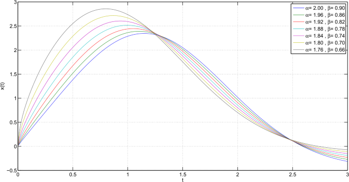

  

  Graph showing $x(t)$ for (6.1) with $\psi (t) = \sin ^{\alpha} (\frac{t}{2} )+\sin ^{\beta} (\frac{t}{3} )$

  Figure 2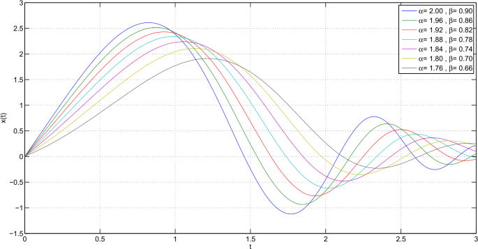

  

  Graph showing $x(t)$ for (6.1) via $\psi (t) = \alpha ^{t} + \beta ^{t}$

  Figure 3

  

  Graph showing $x(t)$ for (6.1) via $\psi (t) = \alpha ^{2}\ln (\beta t+\alpha )$

  Figure 4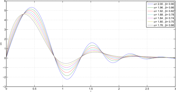

  

  Graph showing $x(t)$ for (6.1) via $\psi (t) = t^{\alpha }+ t^{\beta}$

7 Conclusion

This work examined a novel type of the ψ-Hilfer $\mathbb{PFDE}$s–$\mathbb{MBC}$s, which includes multipoint, fractional derivative multiorder, and fractional integral multiorder $\mathbb{BC}$s. Some properties of the $\mathbb{ML}$ function and fixed-point theory have been employed to effectively obtain the main results. The uniqueness result is investigated by applying the fixed-point theory of Banach type. Furthermore, we demonstrated $\mathbb{U}$–$\mathbb{ML}$ stability in several forms, including $\mathbb{UH}$–$\mathbb{ML}$, $\mathbb{UH}$–$\mathbb{GML}$, $\mathbb{UHR}$–$\mathbb{ML}$, and $\mathbb{UHR}$–$\mathbb{GML}$ stability. Finally, we validated the theoretical conclusions using examples of polynomial, trigonometric, exponential, and logarithmic functions under a variety of functions ψ (see Figures 1–5). In addition, our main results are not only novel in the context of the problem at hand, but they also present some novel particular situations by adjusting the parameters involved. In addition, it is of major significance to note that:

• If we set $\omega _{j} = 0$, $\mu _{k} = 0$ ($j = 1, 2, \ldots , n$, $k = 1, 2, \ldots , r$), in the problem (1.1), our results correspond to those for the nonlinear ψ-Hilfer $\mathbb{PFDE}$s under multipoint $\mathbb{BC}$s.

• If we set $\theta _{i} = 0$, $\mu _{k} = 0$ ($i = 1, 2, \ldots , m$, $k = 1, 2, \ldots , r$), in the problem (1.1), our results correspond to those for the nonlinear ψ-Hilfer $\mathbb{PFDE}$s under fractional integral multiorder $\mathbb{BC}$s.

• If we set $\theta _{i} = 0$, $\omega _{j} = 0$ ($i = 1, 2, \ldots , m$, $j = 1, 2, \ldots , n$), in the problem (1.1), our results correspond to those for the nonlinear ψ-Hilfer $\mathbb{PFDE}$s under fractional derivative multiorder $\mathbb{BC}$s.

Figure 5

Graph showing the functions $f(t,x(t))$

As future work subjects, we will work on the qualitative theory literature on nonlinear fractional $\mathbb{IVP}$s/$\mathbb{BVP}$s involving a special function, like the linear Cauchy-type problem with variable coefficient, stability, or the algorithms to solve the ψ-Hilfer $\mathbb{PFDE}$s/$\mathbb{PFDE}$ systems in mathematical software.

References

Kilbas, A.A., Srivastava, H.M., Trujillo, J.J.: Theory and Applications of Fractional Differential Equations. USA: North-Holland and Mathematics Studies. Elsevier, Amsterdam (2006). https://doi.org/10.1016/s0304-0208(06)x8001-5
Samko, S.G., Kilbas, A.A., Marichev, O.I.: Fractional Integrals and Derivatives: Theory and Applications. Gordon & Breach, Yverdon (1987)
Hilfer, R.: Application of Fractional Calculus in Physics. World Scientific, Singapore (1999)
Magin, R.L.: Fractional Calculus in Bioengineering. Begell House Publishers, USA (2006)
Tarasov, V.E.: Fractional Dynamics: Application of Fractional Calculus to Dynamics of Particles. Fields and Media. Springer, Berlin (2011)
Kilbas, A.A.: Hadamard-type fractional calculus. J. Korean Math. Soc. 38(6), 1191–1204 (2001)
Katugampola, U.N.: New approach to generalized fractional integral. Appl. Math. Comput. 218(3), 860–865 (2011)
Katugampola, U.N.: A new approach to generalized fractional derivatives. Bull. Math. Anal. Appl. 6(4), 1–15 (2014)
Jarad, F., Abdeljawad, T., Baleanu, D.: On the generalized fractional derivatives and their Caputo modification. J. Nonlinear Sci. Appl. 10(5), 2607–2619 (2017)
Jarad, F., Abdeljawad, T., Baleanu, D.: Caputo-type modification of the Hadamard fractional derivative. Adv. Differ. Equ. 2012, 142 (2012)
Jarad, F., Uǵurlu, E., Abdeljawad, T., Baleanu, D.: On a new class of fractional operators. Adv. Differ. Equ. 2018(2018), 142 (2018)
Jarad, F., Abdeljawad, T.: Generalized fractional derivatives and Laplace transform. Discrete Contin. Dyn. Syst. 13(3), 709–722 (2020)
Khalil, R., AlHorani, M., Yousef, A., Sababheh, M.: A new definition of fractional derivative. J. Comput. Appl. Math. 264, 65–70 (2014)
Abdeljawad, T.: On conformable fractional calculus. J. Comput. Appl. Math. 279, 57–66 (2013)
Anderson, D.R., Ulness, D.J.: Newly defined conformable derivatives. Adv. Dyn. Syst. Appl. 10(2), 109–113 (2015)
Anderson, D.R.: Second-order self-adjoint differential equations using a proportionalderivative controller. Commun. Appl. Nonlinear Anal. 24(1), 17–48 (2017)
Jarad, F., Abdeljawad, T., Alzabut, J.: Generalized fractional derivatives generated by a class of local proportional derivatives. Eur. Phys. J. Spec. Top. 226, 3457–3471 (2017). https://doi.org/10.1140/epjst/e2018-00021-7
Alzabut, J., Abdeljawad, T., Jarad, F., Sudsutad, W.: A Gronwall inequality via the generalized proportional fractional derivative with applications. J. Inequal. Appl. 2019, Article ID 101 (2019)
Jarad, F., Alqudah, M.A., Abdeljawad, T.: On more general forms of proportional fractional operators. Open Math. 18, 167–176 (2020). https://doi.org/10.1515/math-2020-0014
Jarad, F., Abdeljawad, T., Rashid, S., Hammouch, Z.: More properties of the proportional fractional integrals and derivatives of a function with respect to another function. Adv. Differ. Equ. 2020, 303 (2020)
Ahmed, I., Kumam, P., Jarad, F., Borisut, P., Jirakitpuwapat, W.: On Hilfer generalized proportional fractional derivative. Adv. Differ. Equ. 2020, 329 (2020). https://doi.org/10.1186/s13662-020-02792-w
Mallah, I., Ahmed, I., Akgul, A., Jarad, F., Alha, S.: On ψ-Hilfer generalized proportional fractional operators. AIMS Math. 7(1), 82–103 (2021). https://doi.org/10.3934/math.2022005
Ulam, S.M.: A Collection of Mathematical Problems. Interscience, New York (1968)
Hyers, D.H.: On the stability of the linear functional equation. Proc. Natl. Acad. Sci. USA 27, 222–224 (1941)
Rassias, T.M.: On the stability of linear mappings in Banach spaces. Proc. Am. Math. Soc. 72, 297–300 (1978)
Wang, J., Li, X.: \(E_{\alpha}\)-Ulam type stability of fractional order ordinary differential equations. J. Appl. Math. Comput. 45, 449–459 (2014). https://doi.org/10.1007/s12190-013-0731-8
Vanterler da C. Sousa, J., de Oliveira, E.C.: A Gronwall inequality and the Cauchy-type problem by means of ψ-Hilfer operator. Differ. Equ. Appl. 11(1), 87–106 (2019)
Liu, K., Wang, J., O’Regan, D.: Ulam–Hyers–Mittag–Leffler stability for ψ-Hilfer fractional-order delay differential equations. Adv. Differ. Equ. 2019, 50 (2019)
Harikrishnan, S., Shak, K., Kanagarajan, K.: Study of a boundary value problem for fractional order ψ-Hilfer fractional derivative. Arab. J. Math., 25 (2019)
Abdo, M.S., Panchal, S.K.: Fractional integro-differential equations involving ψ-Hilfer fractional derivative. Adv. Appl. Math. Mech. 11, 338–359 (2019)
Kucche, K.D., Mali, A.D., Vanterler da C Sousa, J.: On the nonlinear ψ-Hilfer fractional differential equations. Comput. Appl. Math. 38, 73 (2019). https://doi.org/10.1007/s40314-019-0833-5
Almalahi, M.A., Panchal, S.K.: On the theoty of ψ-Hilfer nonlocal Cauchy problem. J. Sib. Fed. Univ. Math. Phys. 14(2), 161–177 (2021). https://doi.org/10.17516/1997-1397-2021-14-2-161-177
Kucche, K.D., Kharade, J.P.: Global existence and Ulam-Hyers stability of ψ-Hilfer fractional differential equations. Kyungpook Math. J. 60(3), 647–671 (2020)
Vanterler da C. Sousa, J., Kucche, K.D., de Oliveira, E.C.: On the Ulam–Hyers stabilities of the solutions of ψ-Hilfer fractional differential equation with abstract Volterra operator. Math. Methods Appl. Sci. 42(9), 3021–3032 (2019)
Vanterler da C Sousa, J., de Oliveira, E.C.: On the Ulam–Hyers–Rassias stability for nonlinear fractional differential equations using the ψ-Hilfer operator. J. Fixed Point Theory Appl. 20(3), 96 (2018)
de Oliveira, E.C., Vanterler da C Sousa, J.: Ulam–Hyers–Rassias stability for a class of fractional integro-differential equations. Results Math. 73, 111 (2018). https://doi.org/10.1007/s00025-018-0872-z
Almalahi, M.A., Panchal, S.K.: Some existence and stability results for ψ-Hilfer fractional implicit diferential equation with periodic conditions. J. Math. Anal. Model. 1(1), 1–19 (2020)
Sudsutad, W., Thaiprayoon, C., Ntouyas, S.K.: Existence and stability results for ψ-Hilfer fractional integro-differential equation with mixed nonlocal boundary conditions. AIMS Math. 6(4), 4119–4141 (2021). https://doi.org/10.3934/math.2021244
Abdo, M.S., Panchal, S.K., Wahash, H.A.: Ulam–Hyers-Mittag-Leffler stability for a ψ-Hilfer problem with fractional order and infinite delay. Results Appl. Math. 7, 100115 (2020). https://doi.org/10.1016/j.rinam.2020.100115
Almalahi, M.A., Abdo, M.S., Panchal, S.K.: Existence and Ulam–Hyers–Mittag–Leffler stability results of Ψ-Hilfer nonlocal Cauchy problem. Rend. Circ. Mat. Palermo 70(1), 57–77 (2020). https://doi.org/10.1007/s12215-020-00484-8
Boucenna, D., Baleanu, D., Makhlouf, A.B., Nagy, A.M.: Analysis and numerical solution of the generalized proportional fractional Cauchy problem. Appl. Numer. Math. 167, 173–186 (2021)
Khaminsou, B., Sudsutad, W., Thaiprayoon, C., Alzabut, J., Pleumpreedaporn, S.: Analysis of impulsive boundary value pantograph problems via Caputo proportional fractional derivative under Mittag–Leffler functions. Fractal Fract. 5, 251 (2021). https://doi.org/10.3390/fractalfract5040251
Alzabut, J., Adjabi, Y., Sudsutad, W., Rehman, M.-U.: New generalizations for Gronwall type inequalities involving a ψ-fractional operator and their applications. AIMS Math. 6(5), 5053–5077 (2021). https://doi.org/10.3934/math.2021299
Younus, A., Asif, M., Alzabut, J., Ghaffar, A., Sooppy Nisar, K.: Improved interval-valued Gronwall type inequalities. Adv. Differ. Equ. 2020, 319 (2020). https://doi.org/10.1186/s13662-020-02781-z
Alzabut, J., Sudsutad, W., Kayar, Z., Baghani, H.: A new Gronwall-Bellman inequality in frame of generalized proportional fractional derivative. Mathematics 7(8), 747 (2019)
Alzabut, J., Abdeljawad, T.: A generalized discrete fractional Gronwall’s inequality and its application on the uniqueness of solutions for nonlinear delay fractional difference system. Appl. Anal. Discrete Math. 12, 036 (2018)
Wang, J.R., Feckan, M., Zhou, Y.: Presentation of solutions of impulsive fractional Langevin equations and existence results. Eur. Phys. J. Spec. Top. 222(8), 1857–1874 (2013)
Courant, R.: Differential and Integral Calculus, vol. 2. Wiley, New York (2011)
Lima, E.L.: Real Analysis. Instituto de Matemática Pura e Aplicada, CNPq, Rio de Janeiro (2004). (in portuguese)
Wong, R.: Asymptotic Approximations of Integrals. SIAM, Philadelphia (2001)
Ashyraliyev, M.: On Gronwall’s type integral inequalities with singular kernels. Filomat 31(4), 1041–1049 (2017)
Ye, H., Gao, J., Ding, Y.: A generalized Gronwall inequality and its application to a fractional differential equation. J. Math. Anal. Appl. 328(2), 1075–1081 (2007)
Gong, Z., Qian, D., Li, C., Guo, P.: On the Hadamard type fractional differential system. In: Frac. Dyn. Control, pp. 159–171. Springer, New York (2012)
Deimling, K.: Nonlinear Functional Analysis. Springer, New York (1985)
Acknowledgements
W. Sudsutad was partially supported by Ramkhamhaeng University. C. Thaiprayoon and J. Kongson would like to thank Burapha University for funding and support. J. Alzabut would like to thank Prince Sultan University and OSTİM Technical University for supporting this research.
Funding
Not applicable.
Author information
Authors and Affiliations
Contributions
WS: problem statement, conceptualization, methodology, investigation, writing the original draft, writing, reviewing, and editing, funding acquisition. CT, BK: methodology, investigation, writing, reviewing, and editing. JA: supervision. JK: investigation, writing, reviewing, and editing, funding acquisition. All the authors read and approved the final manuscript.
Corresponding author
Ethics declarations
Competing interests
The authors declare that they have no competing interests.
Rights and permissions
Open Access This article is licensed under a Creative Commons Attribution 4.0 International License, which permits use, sharing, adaptation, distribution and reproduction in any medium or format, as long as you give appropriate credit to the original author(s) and the source, provide a link to the Creative Commons licence, and indicate if changes were made. The images or other third party material in this article are included in the article’s Creative Commons licence, unless indicated otherwise in a credit line to the material. If material is not included in the article’s Creative Commons licence and your intended use is not permitted by statutory regulation or exceeds the permitted use, you will need to obtain permission directly from the copyright holder. To view a copy of this licence, visit http://creativecommons.org/licenses/by/4.0/.
About this article
Cite this article
Sudsutad, W., Thaiprayoon, C., Khaminsou, B. et al. A Gronwall inequality and its applications to the Cauchy-type problem under ψ-Hilfer proportional fractional operators. J Inequal Appl 2023, 20 (2023). https://doi.org/10.1186/s13660-023-02929-x
Received:
Accepted:
Published:
DOI: https://doi.org/10.1186/s13660-023-02929-x