On convexity analysis for discrete delta Riemann–Liouville fractional differences analytically and numerically

Abstract

In this paper, we focus on the analytical and numerical convexity analysis of discrete delta Riemann–Liouville fractional differences. In the analytical part of this paper, we give a new formula for the discrete delta Riemann-Liouville fractional difference as an alternative definition. We establish a formula for the $\Delta ^{2}$, which will be useful to obtain the convexity results. We examine the correlation between the positivity of $({}^{\mathrm{RL}}_{w_{0}}\Delta ^{\alpha} \mathrm{f} )( \mathrm{t})$ and convexity of the function. In view of the basic lemmas, we define two decreasing subsets of $(2,3)$, $\mathscr{H}_{\mathrm{k},\epsilon}$ and $\mathscr{M}_{\mathrm{k},\epsilon}$. The decrease of these sets allows us to obtain the relationship between the negative lower bound of $({}^{\mathrm{RL}}_{w_{0}}\Delta ^{\alpha} \mathrm{f} )( \mathrm{t})$ and convexity of the function on a finite time set $\mathrm{N}_{w_{0}}^{\mathrm{P}}:=\{w_{0}, w_{0}+1, w_{0}+2,\dots , \mathrm{P}\}$ for some $\mathrm{P}\in \mathrm{N}_{w_{0}}:=\{w_{0}, w_{0}+1, w_{0}+2,\dots \}$. The numerical part of the paper is dedicated to examinin the validity of the sets $\mathscr{H}_{\mathrm{k},\epsilon}$ and $\mathscr{M}_{\mathrm{k},\epsilon}$ for different values of k and ϵ. For this reason, we illustrate the domain of solutions via several figures explaining the validity of the main theorem.

1 Introduction

The recent development of pure and applied mathematics is characterized by increasing attempts to use mathematical modeling tools of fractional order in different engineering, medicinal, and biological fields. It is known that this mathematical modeling of fractional order attempts to improve our understanding of more and more complicated phenomena, and in general, it is based on ordinary and partial differential equations. In the past several decades, some algorithms have been proposed for solving such fractional problems, which can be classified into different categories (see [1–4]).

Discrete fractional problems and discrete fractional operators are worth studying in the setting of fractional calculus and have attracted much attention from scholars. Furthermore, the concept of discrete fractional calculus was rooted in the few decades; it gets attention of many researchers recently because of their inquisitive thinking (see [5–7] and references therein). The main reason is that these problems and operators have a wide range of practical applications, such as mathematical analysis [8, 9], stability analysis [10–12], probability and statistics [13–15], geometry [16, 17], ecology [18, 19], and topology [20–22].

Positivity, monotonicity and convexity analysis plays a crucial role in discrete fractional calculus theory. Although a number of papers have been contributed to the analysis of discrete fractional operators with singular and nonsingular kernel type, the question of positivity, monotonicity, and convexity of discrete fractional operators of Riemann–Liouville type on a time set still remains open. Furthermore, the positivity, monotonicity, and convexity analysis is important in understanding the nature of the discrete fractional problems from the perspective of continuous fractional problems. Many authors have developed many interesting results on optimality and duality in the setting of Riemann–Liouville and Liouville–Caputo fractional differences; see, for instance, [5, 23–26] and the references therein.

Let $\mathrm{N}_{w_{0}}:=\{w_{0},w_{0}+1,w_{0}+2,\ldots \}$ and ${{\mathscr{G}_{w_{0}}(\mathrm{f}):=\{ \mathrm{f}:\mathrm{N}_{w_{0}}\rightarrow \mathcal{R}\text{ for } w_{0}\in \mathcal{R} \}}}$. There is a clean and clear correlation between the convexity of a function $\mathrm{f}\in \mathscr{G}_{w_{0}}(\mathrm{f})$ and the nonnegativity of the $\Delta ^{2}$ difference of f, given in the following relationship:

$$\begin{aligned} \text{If } \bigl(\Delta ^{2}\mathrm{f} \bigr) (\mathrm{t})\geq 0, \quad \text{then we say that } \mathrm{f} \text{ is convex at } \mathrm{t}. \end{aligned}$$

Particularly, convexity has been studied in fractional calculus quite extensively. However, with discrete fractional calculus theory and discrete operators, this area has not received a lot of attention so far. Moreover, in terms of numerical simulations, some works can be found for monotonicity analysis of the discrete fractional calculus operators (see [27–29] and references therein) or convexity analysis of these operators (see [30–32] and references therein).

The main objective of this paper is to provide a relationship between the positive lower bound of the fractional difference operators of delta Riemann–Lioville type $({}^{\mathrm{RL}}_{w_{0}}\Delta ^{\alpha} \mathrm{f} )( \mathrm{t})$ and the convexity of a function f on an infinite time set $\mathrm{N}_{w_{0}}$ and a relationship between the negative lower bound of $({}^{\mathrm{RL}}_{w_{0}}\Delta ^{\alpha} \mathrm{f} )( \mathrm{t})$ and convexity of a function f on a finite time set $\mathrm{N}_{w_{0}}^{\mathrm{P}}$. Besides, we present some numerical simulations for the negative lower bound case to demonstrate the solution spaces of the defined sets on the negative lower boundedness of $({}^{\mathrm{RL}}_{w_{0}}\Delta ^{\alpha} \mathrm{f} )( \mathrm{t})$.

The paper is organized as follows. Section 2 contains main properties and notations of discrete fractional operators of delta Riemann–Lioville type. In Sect. 3, we state and prove our analytical results by defining the sets $\mathscr{H}_{\mathrm{k},\epsilon}$ and $\mathscr{M}_{\mathrm{k},\epsilon}$, studying the main lemmas and theorems on the sets, and examining the delta convexity results of the proposed difference operators. Section 4 deals with numerical results including eight illustrative figures, in which the time steps will be applied on the sets $\mathscr{H}_{\mathrm{k},\epsilon}$ and $\mathscr{M}_{\mathrm{k},\epsilon}$ as applications. Also, the domains of the solutions are determined for both sets. Finally, in Sect. 5, we provide a conclusion along with future work possibilities in this field.

2 Basic tools and results

In this section, we briefly consider the discrete fractional sums and differences in the setting of Riemann–Liouville. We refer the reader to [5, 12, 33, 34] for the relevant details.

For $\mathrm{f}\in \mathscr{G}_{w_{0}+\alpha}(\mathrm{f})$ with $\alpha >0$, the Δ sum operator of order α can be defined as follows:

$$\begin{aligned} \bigl({}_{w_{0}}\Delta ^{-\alpha}\mathrm{f} \bigr) ( \mathrm{t})&=\frac{1}{\Gamma (\alpha )}\sum_{\mathrm{s}=w_{0}}^{ \mathrm{t}-\alpha} (\mathrm{t}-1-\mathrm{s} )^{ \underline{\alpha -1}}\mathrm{f}(\mathrm{s}) \quad \text{for } \mathrm{t} \text{ in } \mathrm{N}_{w_{0}+\alpha}, \end{aligned}$$

(2.1)

where $\mathrm{t}^{\underline{\alpha}}$ is defined by

$$\begin{aligned} \mathrm{t}^{\underline{\alpha}} = \frac{\Gamma (1+\mathrm{t} )}{\Gamma (1+\mathrm{t}-\alpha )}, \end{aligned}$$

(2.2)

such that the right-hand side of this identity is well defined. Besides, we use $\mathrm{t}^{\underline{\alpha}}=0$ when the numerators in each identity is well-defined but the denominator is not. Further, we have

$$ \Delta \mathrm{t}^{\underline{\alpha}}=\alpha \mathrm{t}^{ \underline{\alpha -1}}. $$

(2.3)

Definition 2.1

(see [5, 33, 34])

Let $\mathrm{f}\in \mathscr{G}_{w_{0}}(\mathrm{f})$. Then $(\Delta \mathrm{f} )(\mathrm{t}):=\mathrm{f}( \mathrm{t}+1)-\mathrm{f}(\mathrm{t})$ for $\mathrm{t}\in \mathrm{N}_{w_{0}}$ is the Δ difference operator. In addition, the Δ fractional difference of order α ($\aleph -1< \alpha <\aleph$) of the Riemann–Liouville type is defined by

$$\begin{aligned} \bigl({}^{\mathrm{RL}}_{w_{0}}\Delta ^{\alpha} \mathrm{f} \bigr) ( \mathrm{t}) &=\frac{\Delta ^{\aleph}}{\Gamma (\aleph -\alpha )} \sum _{ \mathrm{s}=w_{0}}^{\mathrm{t}+\alpha -\aleph} (\mathrm{t}- \mathrm{s}-1 )^{\underline{\aleph -\alpha -1}}\mathrm{f}( \mathrm{s}) \quad \text{for } \mathrm{t} \text{ in } \mathrm{N}_{w_{0}+ \aleph -\alpha}. \end{aligned}$$

(2.4)

The following theorem is an alternative representation of the Δ fractional difference (2.4), which is also a generalization of the result established for $0<\alpha <1$ in [25].

Theorem 2.1

For $\mathrm{f}\in \mathscr{G}_{w_{0}+\alpha}(\mathrm{f})$ with $\aleph -1<\alpha <\aleph$, the Δ fractional difference of order α of the Riemann–Liouville type can be given by

$$\begin{aligned} \bigl({}^{\mathrm{RL}}_{w_{0}}\Delta ^{\alpha} \mathrm{f} \bigr) ( \mathrm{t}) =\frac{1}{\Gamma (-\alpha )} \sum _{\mathrm{s}=w_{0}}^{ \mathrm{t}+\alpha}(\mathrm{t} -\mathrm{s}-1)^{\underline{-\alpha -1}} \mathrm{f}(\mathrm{s}) \quad \textit{for } \mathrm{t} \textit{ in } \mathrm{N}_{w_{0}+\aleph -\alpha}. \end{aligned}$$

(2.5)

Proof

The result was proved by Mohammed et al. [25, Theorem 1] for $\aleph =1$ (that is, for $0<\alpha <1$), and their result is

$$\begin{aligned} \bigl({}^{\mathrm{RL}}_{w_{0}}\Delta ^{\alpha}\mathrm{f} \bigr) ( \mathrm{t})=\frac{1}{\Gamma (-\alpha )} \sum _{\mathrm{s}=w_{0}}^{ \mathrm{t}+\alpha}(\mathrm{t}- \mathrm{s}-1)^{\underline{-\alpha -1}} \mathrm{f}(\mathrm{s}) \quad \text{for } \mathrm{t} \text{ in } \mathrm{N}_{w_{0}+1-\alpha}. \end{aligned}$$

(2.6)

For $\aleph =2$ (that is, for $1<\alpha <2$), by Definition (2.4) we find that for each $\mathrm{t}\in \mathrm{N}_{w_{0}+2-\alpha}$,

$$\begin{aligned} \bigl({}^{\mathrm{RL}}_{w_{0}}\Delta ^{\alpha}\mathrm{f} \bigr) ( \mathrm{t}) &=\Delta ^{2} \Biggl(\frac{1}{\Gamma (-\alpha +2)}\sum _{ \mathrm{s}=w_{0}}^{\mathrm{t}+\alpha -2} (\mathrm{t}-\mathrm{s}-1 )^{\underline{1-\alpha}}\mathrm{f}(\mathrm{s}) \Biggr) \\ &\overset{\text{by}}{\underset{\text{(2.6)}}{=}} \Delta \Biggl( \frac{1}{\Gamma (-\alpha +1)}\sum_{\mathrm{s}=w_{0}}^{\mathrm{t}+ \alpha -1} ( \mathrm{t}-\mathrm{s}-1 )^{\underline{-\alpha}} \mathrm{f}(\mathrm{s}) \Biggr) \\ &=\frac{1}{\Gamma (-\alpha +1)} \Biggl\{ \sum_{\mathrm{s}=w_{0}}^{ \mathrm{t}+\alpha} (\mathrm{t}-\mathrm{s} )^{ \underline{-\alpha}}\mathrm{f}(\mathrm{s}) -\sum _{\mathrm{s}=w_{0}}^{ \mathrm{t}+\alpha -1} (\mathrm{t}-\mathrm{s}-1 )^{ \underline{-\alpha}}\mathrm{f}(\mathrm{s}) \Biggr\} \\ &=\frac{1}{\Gamma (-\alpha +1)} \Biggl\{ \sum_{\mathrm{s}=w_{0}}^{ \mathrm{t}+\alpha} (\mathrm{t}-\mathrm{s} )^{ \underline{-\alpha}}\mathrm{f}(\mathrm{s}) -\sum _{\mathrm{s}=w_{0}}^{ \mathrm{t}+\alpha} (\mathrm{t}-\mathrm{s}-1 )^{ \underline{-\alpha}}\mathrm{f}(\mathrm{s}) \Biggr\} \\ &=\frac{1}{\Gamma (-\alpha +1)}\sum_{\mathrm{s}=w_{0}}^{\mathrm{t}+ \alpha} \Delta (\mathrm{t}-\mathrm{s}-1 )^{ \underline{-\alpha}}\mathrm{f}(\mathrm{s}) \\ &=\frac{1}{\Gamma (-\alpha )} \sum_{\mathrm{s}=w_{0}}^{\mathrm{t}+ \alpha}( \mathrm{t}-\mathrm{s}-1)^{\underline{-\alpha -1}}\mathrm{f}( \mathrm{s}), \end{aligned}$$

where we have first used (see [25, Lemma 1])

$$ (-\alpha -1 )^{\underline{-\alpha}}=0 $$

and then used

$$ \Delta \bigl(\mathrm{t}^{\underline{-\alpha}} \bigr) =-\alpha \mathrm{t}^{\underline{-\alpha -1}}. $$

The same procedure can be repeated $\aleph -1$ times to obtain the required result stated by Theorem 2.1. □

3 Negative lower bound results

Let us state and prove our main lemma concerning the $\Delta ^{2}$ fractional difference.

Lemma 3.1

Let $\mathrm{f}\in \mathscr{G}_{w_{0}}(\mathrm{f})$, $\alpha \in (2,3)$, and $({}^{\mathrm{RL}}_{w_{0}}\Delta ^{\alpha}\mathrm{f} )( \mathrm{t})\geqq 0$ for $\mathrm{t}\in \mathrm{N}_{w_{0}+3-\alpha}$. Then, for $\mathrm{t}:=w_{0}-\alpha +3+\mathrm{k}$ with $\mathrm{k}\in \mathrm{N}_{0}$,

$$\begin{aligned} \bigl(\Delta ^{2} \mathrm{f} \bigr) (w_{0}+\mathrm{k}+1)\geqq - \frac{ (-\alpha +3+\mathrm{k} )^{\underline{-\alpha}}}{\Gamma (-\alpha +1)} \mathrm{f}(w_{0})- \frac{ (-\alpha +3+\mathrm{k} )^{\underline{1-\alpha}}}{\Gamma (-\alpha +2)} (\Delta \mathrm{f} ) (w_{0}) \\ \quad {}-\frac{1}{\Gamma (-\alpha +2)}\sum_{\imath =0}^{\mathrm{k}} (- \alpha +\mathrm{k}+2-\imath )^{\underline{1-\alpha}} \bigl( \Delta ^{2} \mathrm{f} \bigr) (w_{0}+\imath ), \end{aligned}$$

(3.1)

where

$$\begin{aligned} \frac{ (-\alpha +\mathrm{k}+2-\imath )^{\underline{1-\alpha}}}{\Gamma (-\alpha +2)} = \frac{(-\alpha +2)(-\alpha +3)\cdots (-\alpha +\mathrm{k}+2-\imath )}{(\mathrm{k}-\imath +1)!}< 0 \end{aligned}$$

(3.2)

and

$$\begin{aligned} \frac{ (-\alpha +3+\mathrm{k} )^{\underline{-\alpha}}}{\Gamma (-\alpha +1)}>0 \quad \textit{and}\quad \frac{ (-\alpha +3+\mathrm{k} )^{\underline{1-\alpha}}}{\Gamma (-\alpha +2)}< 0. \end{aligned}$$

(3.3)

Proof

By Theorem 2.1 and (2.3) we have

$$\begin{aligned} \begin{aligned} \bigl({}^{\mathrm{RL}}_{w_{0}}\Delta ^{\alpha}\mathrm{f} \bigr) ( \mathrm{t})&=\frac{1}{\Gamma (-\alpha )} \sum_{\mathrm{s}=w_{0}}^{ \mathrm{t}+\alpha}( \mathrm{t}-\mathrm{s}-1)^{\underline{-\alpha -1}} \mathrm{f}(\mathrm{s}) \\ &=\frac{1}{\Gamma (-\alpha +1)} \sum_{\mathrm{s}=w_{0}}^{\mathrm{t}+ \alpha} \Delta (\mathrm{t}-\mathrm{s}-1)^{\underline{-\alpha}} \mathrm{f}(\mathrm{s}) \\ &= \frac{(\mathrm{t}-w_{0})^{\underline{-\alpha}}}{\Gamma (-\alpha +1)} \mathrm{f}(w_{0}) +\frac{1}{\Gamma (-\alpha +1)} \sum_{\mathrm{s}=w_{0}}^{ \mathrm{t}+\alpha}(\mathrm{t}- \mathrm{s}-1)^{\underline{-\alpha}} (\Delta \mathrm{f} ) (\mathrm{s}), \end{aligned} \end{aligned}$$

where we have used $(-\alpha -1)^{\underline{-\alpha}}=0$. By the same technique as before, we can deduce

$$\begin{aligned} \bigl({}^{\mathrm{RL}}_{w_{0}}\Delta ^{\alpha}\mathrm{f} \bigr) ( \mathrm{t}) &= \frac{(\mathrm{t}-w_{0})^{\underline{-\alpha}}}{\Gamma (-\alpha +1)} \mathrm{f}(w_{0})+\frac{1}{\Gamma (-\alpha +2)} \sum _{\mathrm{s}=w_{0}}^{ \mathrm{t}+\alpha}\Delta (\mathrm{t}- \mathrm{s}-1)^{ \underline{1-\alpha}} (\Delta \mathrm{f} ) (\mathrm{s}) \\ &= \frac{(\mathrm{t}-w_{0})^{\underline{-\alpha}}}{\Gamma (-\alpha +1)} \mathrm{f}(w_{0}) + \frac{(\mathrm{t}-w_{0})^{\underline{1-\alpha}}}{\Gamma (-\alpha +2)} (\Delta \mathrm{f} ) (w_{0}) \\ &\quad {}+\frac{1}{\Gamma (-\alpha +2)} \sum _{\mathrm{s}=w_{0}}^{\mathrm{t}+\alpha}(\mathrm{t}-\mathrm{s}-1)^{ \underline{1-\alpha}} \bigl(\Delta ^{2} \mathrm{f} \bigr) (\mathrm{s}), \end{aligned}$$

(3.4)

where we have used $(-\alpha -1)^{\underline{1-\alpha}}=0$. Since $(\mathrm{t}-\mathrm{s}-1)^{\underline{1-\alpha}}=0$ at $\mathrm{s}=\mathrm{t}+\alpha , \mathrm{t}+\alpha -1$, (3.4) becomes

$$\begin{aligned} \bigl({}^{\mathrm{RL}}_{w_{0}}\Delta ^{\alpha}\mathrm{f} \bigr) ( \mathrm{t}) &= \frac{(\mathrm{t}-w_{0})^{\underline{-\alpha}}}{\Gamma (-\alpha +1)} \mathrm{f}(w_{0})+ \frac{(\mathrm{t}-w_{0})^{\underline{1-\alpha}}}{\Gamma (-\alpha +2)} (\Delta \mathrm{f} ) (w_{0}) \\ &\quad {} +\frac{1}{\Gamma (-\alpha +2)} \sum_{\mathrm{s}=w_{0}}^{\mathrm{t}+\alpha -2}( \mathrm{t}-\mathrm{s}-1)^{ \underline{1-\alpha}} \bigl(\Delta ^{2}\mathrm{f} \bigr) (\mathrm{s}) \\ &= \bigl(\Delta ^{2}\mathrm{f} \bigr) (\mathrm{t}+\alpha -2) + \frac{(\mathrm{t}-w_{0})^{\underline{-\alpha}}}{\Gamma (-\alpha +1)} \mathrm{f}(w_{0}) + \frac{(\mathrm{t}-w_{0})^{\underline{1-\alpha}}}{\Gamma (-\alpha +2)} ( \Delta \mathrm{f} ) (w_{0}) \\ &\quad{}+ \frac{1}{\Gamma (-\alpha +2)}\sum_{\mathrm{s}=w_{0}}^{\mathrm{t}+ \alpha -3}( \mathrm{t}-\mathrm{s}-1)^{\underline{1-\alpha}} \bigl( \Delta ^{2}\mathrm{f} \bigr) (\mathrm{s}). \end{aligned}$$

(3.5)

By the assumption $({}^{\mathrm{RL}}_{w_{0}}\Delta ^{\alpha}\mathrm{f} )( \mathrm{t})\geqq 0$ it follows that

$$\begin{aligned} \bigl(\Delta ^{2}\mathrm{f} \bigr) (\mathrm{t}+\alpha -2) \geqq& - \frac{(\mathrm{t}-w_{0})^{\underline{-\alpha}}}{\Gamma (-\alpha +1)} \mathrm{f}(w_{0}) - \frac{(\mathrm{t}-w_{0})^{\underline{1-\alpha}}}{\Gamma (-\alpha +2)} ( \Delta \mathrm{f} ) (w_{0}) \\ &{} -\frac{1}{\Gamma (-\alpha +2)} \sum _{\mathrm{s}=w_{0}}^{\mathrm{t}+\alpha -3}(\mathrm{t}-\mathrm{s}-1)^{ \underline{1-\alpha}} \bigl(\Delta ^{2}\mathrm{f} \bigr) (\mathrm{s}). \end{aligned}$$

For $\mathrm{t}:=w_{0}-\alpha +3+\mathrm{k}$ with $\mathrm{k}\in \mathrm{N}_{0}$, it becomes

$$\begin{aligned} \bigl(\Delta ^{2}\mathrm{f} \bigr) (w_{0}+\mathrm{k}+1) \geqq& - \frac{(-\alpha +3+\mathrm{k})^{\underline{-\alpha}}}{\Gamma (-\alpha +1)} \mathrm{f}(w_{0}) - \frac{(-\alpha +3+\mathrm{k})^{\underline{1-\alpha}}}{\Gamma (-\alpha +2)} (\Delta \mathrm{f} ) (w_{0}) \\ & {}-\frac{1}{\Gamma (-\alpha +2)}\sum_{\imath =0}^{\mathrm{k}}(2- \alpha +\mathrm{k}-\imath )^{\underline{1-\alpha}} \bigl(\Delta ^{2} \mathrm{f} \bigr) (w_{0}+\imath ), \end{aligned}$$

which is the required (3.1). Now it is clear that for $2<\alpha <3$,

$$\begin{aligned}& \begin{aligned} \frac{ (-\alpha +\mathrm{k}+2-\imath )^{\underline{1-\alpha}}}{\Gamma (-\alpha +2)} &= \frac{\Gamma (-\alpha +3+\mathrm{k}-\imath )}{\Gamma (-\alpha +2)\Gamma (2+\mathrm{k}-\imath )} \\ &= \frac{(-\alpha +2)(-\alpha +3)\cdots (-\alpha +\mathrm{k}+2-\imath )}{(\mathrm{k}-\imath +1)!}< 0, \end{aligned} \\& \begin{aligned} \frac{ (-\alpha +3+\mathrm{k} )^{\underline{-\alpha}}}{\Gamma (-\alpha +1)} &= \frac{\Gamma (-\alpha +4+\mathrm{k})}{\Gamma (4+\mathrm{k})\Gamma (-\alpha +1)} \\ &= \frac{(-\alpha +1)(-\alpha +2)(-\alpha +3)\cdots (-\alpha +\mathrm{k}+1)(-\alpha +\mathrm{k}+2)(-\alpha +\mathrm{k}+3)}{(\mathrm{k}+3)!} \\ &>0, \end{aligned} \end{aligned}$$

and

$$\begin{aligned} \frac{ (-\alpha +3+\mathrm{k} )^{\underline{1-\alpha}}}{\Gamma (-\alpha +2)} &= \frac{\Gamma (-\alpha +4+\mathrm{k})}{\Gamma (4+\mathrm{k})\Gamma (-\alpha +2)} \\ &= \frac{(-\alpha +2)(-\alpha +3)\cdots (-\alpha +\mathrm{k}+2)(-\alpha +\mathrm{k}+3)}{(\mathrm{k}+3)!}< 0 \end{aligned}$$

for $\imath =0, 1,\ldots ,\mathrm{k}$ and $\mathrm{k}\in \mathrm{N}_{0}$. Thus our proof is complete. □

Based on this lemma, we now can present the Δ convexity result.

Theorem 3.1

If $\alpha \in (2,3)$ and $\mathrm{f}\in \mathscr{G}_{w_{0}}(\mathrm{f})$ satisfies $({}^{\mathrm{RL}}_{w_{0}}\Delta ^{\alpha}\mathrm{f} )( \mathrm{t})\geqq 0$ for all $\mathrm{t}\in \mathrm{N}_{w_{0}+3-\alpha}$, $\mathrm{f}(w_{0})\leqq 0$, $(\Delta \mathrm{f})(w_{0})\geqq 0$, and $(\Delta ^{2} \mathrm{f} )(w_{0})\geqq 0$, then $(\Delta ^{2} \mathrm{f} )(\mathrm{t})\geqq 0$ for $\mathrm{t}\in \mathrm{N}_{w_{0}}$.

Proof

We will prove by using strong induction. From the assumption we know that $(\Delta ^{2} \mathrm{f} )(w_{0})\geqq 0$. We assume that $(\Delta ^{2} \mathrm{f} )(w_{0}+\imath )\geqq 0$ for $\imath =0,1,\ldots ,\mathrm{k}$. Then Lemma 3.1 gives that $(\Delta ^{2} \mathrm{f} )(w_{0}+\mathrm{k}+1)\geqq 0$. Thus the proof is done. □

This theorem has demonstrated a correlation between the nonnegativity of $({}^{\mathrm{RL}}_{w_{0}}\Delta ^{\alpha}\mathrm{f} )( \mathrm{t})$ and the convexity of f. Now we wish to investigate what happens by replacing the zero lower bound of Theorem 3.1 with a negative lower bound −ϵ for some $\epsilon >0$.

Firstly, we need a lemma concerning the sets $\mathscr{H}_{\mathrm{k},\epsilon}$ and $\mathscr{M}_{\mathrm{k},\epsilon}$ defined by

$$\begin{aligned} \mathscr{H}_{\mathrm{k},\epsilon} :=\biggl\{ \alpha \in (2,3); \frac{\Gamma (-\alpha +\mathrm{k}+4)}{\Gamma (-\alpha +1)(\mathrm{k}+3)!} \geqq \epsilon \biggr\} \subseteq (2,3) \end{aligned}$$

(3.6)

and

$$\begin{aligned} \mathscr{M}_{\mathrm{k},\epsilon} :=\biggl\{ \alpha \in (2,3); \frac{\Gamma (-\alpha +\mathrm{k}+4)}{\Gamma (-\alpha +2)(\mathrm{k}+2)!} \leqq -\epsilon \biggr\} \subseteq (2,3), \end{aligned}$$

(3.7)

respectively, for some $\epsilon >0$ and $\mathrm{k}\in \mathrm{N}_{0}$.

Lemma 3.2

The collections $\{\mathscr{H}_{\mathrm{k},\epsilon} \}_{\mathrm{k}=0}^{ \infty}$ and $\{\mathscr{M}_{\mathrm{k},\epsilon} \}_{\mathrm{k}=0}^{ \infty}$ are decreasing for all $\epsilon >0$. Moreover,

$$\begin{aligned} \bigcap_{\mathrm{k}=0}^{\infty}\mathscr{H}_{\mathrm{k},\epsilon}= \emptyset \quad \textit{and}\quad \bigcap_{\mathrm{k}=0}^{\infty} \mathscr{M}_{\mathrm{k},\epsilon}=\emptyset . \end{aligned}$$

Proof

Suppose that $\alpha \in \mathscr{H}_{\mathrm{k}+1,\epsilon}$. Then we have

$$\begin{aligned} & \frac{(-\alpha +\mathrm{k}+4)(-\alpha +\mathrm{k}+3)(-\alpha +\mathrm{k}+2)\cdots (-\alpha +3)(-\alpha +2)(-\alpha +1)}{(\mathrm{k}+3)!} \\ &\quad = \frac{\Gamma (-\alpha +\mathrm{k}+5)}{\Gamma (-\alpha +1)(\mathrm{k}+4)!} \geqq \epsilon . \end{aligned}$$

Also, we know that

$$\begin{aligned} & \frac{\Gamma (-\alpha +\mathrm{k}+5)}{\Gamma (-\alpha +1)(\mathrm{k}+4)!} \\ &\quad =\frac{-\alpha +\mathrm{k}+4}{\mathrm{k}+4} \frac{(-\alpha +\mathrm{k}+3)(-\alpha +\mathrm{k}+2)(-\alpha +\mathrm{k}+1)\cdots (-\alpha +3)(-\alpha +2)(-\alpha +1)}{(\mathrm{k}+3)!} \\ &\quad \leqq \frac{(-\alpha +\mathrm{k}+3)(-\alpha +\mathrm{k}+2)(-\alpha +\mathrm{k}+1)\cdots (-\alpha +3)(-\alpha +2)(-\alpha +1)}{(\mathrm{k}+3)!} \\ &\quad = \frac{\Gamma (-\alpha +\mathrm{k}+4)}{\Gamma (-\alpha +1)(\mathrm{k}+3)!}, \end{aligned}$$

since $\alpha \in (2,3)$,

$$\begin{aligned} \frac{-\alpha +\mathrm{k}+4}{\mathrm{k}+4}\leqq 1 \quad \Longleftrightarrow \quad -\alpha + \mathrm{k}+4 \leqq \mathrm{k}+4 \quad \text{(which is clearly true)}, \end{aligned}$$

and by Lemma 3.1,

$$\begin{aligned} \frac{(-\alpha +\mathrm{k}+3)(-\alpha +\mathrm{k}+2)(-\alpha +\mathrm{k}+1)\cdots (-\alpha +3)(-\alpha +2)(-\alpha +1)}{(\mathrm{k}+3)!} \geqq 0. \end{aligned}$$

Thus $\mathscr{H}_{\mathrm{k}+1,\epsilon} \subseteq \mathscr{H}_{ \mathrm{k},\epsilon}$, and hence the collection $\{\mathscr{H}_{\mathrm{k},\epsilon} \}_{\mathrm{k}=0}^{ \infty}$ is decreasing.

Similarly to the above proof, we can prove that $\{\mathscr{H}_{\mathrm{k},\epsilon} \}_{\mathrm{k}=0}^{ \infty}$ is decreasing as well.

To end the lemma, following Theorem 3.4-1 in [35], we have

$$\begin{aligned} \lim_{\mathrm{k}\to \infty} \frac{\Gamma (-\alpha +\mathrm{k}+4)}{\Gamma (-\alpha +1)(\mathrm{k}+3)!} &=\lim _{\mathrm{k}\to \infty} \frac{\Gamma (-\alpha +\mathrm{k}+4)}{\Gamma (-\alpha +1)\Gamma (\mathrm{k}+4)} \cdot \frac{(\mathrm{k}+4)^{-\alpha}}{(\mathrm{k}+4)^{-\alpha}} \\ &=\lim_{\mathrm{k}\to \infty} \frac{1}{(\mathrm{k}+4)^{\alpha}\Gamma (-\alpha +1)} \cdot \lim _{ \mathrm{k}\to \infty} \frac{\Gamma (-\alpha +\mathrm{k}+4)}{\Gamma (\mathrm{k}+4)}( \mathrm{k}+4)^{\alpha} \\ &=0\cdot 1=0 \end{aligned}$$

(3.8)

and

$$\begin{aligned} \lim_{\mathrm{k}\to \infty} \frac{\Gamma (-\alpha +\mathrm{k}+4)}{\Gamma (-\alpha +2)(\mathrm{k}+2)!} &=\lim _{\mathrm{k}\to \infty} \frac{\Gamma (-\alpha +\mathrm{k}+4)}{\Gamma (-\alpha +2)\Gamma (\mathrm{k}+3)} \cdot \frac{(\mathrm{k}+3)^{-\alpha}}{(\mathrm{k}+3)^{-\alpha}} \\ &=\lim_{\mathrm{k}\to \infty} \frac{1}{(\mathrm{k}+3)^{\alpha}\Gamma (-\alpha +2)} \cdot \lim _{ \mathrm{k}\to \infty} \frac{\Gamma (-\alpha +\mathrm{k}+4)}{\Gamma (\mathrm{k}+3)}( \mathrm{k}+3)^{\alpha} \\ &=0\cdot 1=0. \end{aligned}$$

(3.9)

Hence, for $\epsilon >0$, there exist $\mathrm{k}_{1}:=\mathrm{k}_{1}(\epsilon )\geqq 0$ and $\mathrm{k}_{2}:=\mathrm{k}_{2}(\epsilon )\geqq 0$ such that $\mathscr{H}_{\mathrm{k},\epsilon}=\emptyset$ for all $\mathrm{k}\geqq \mathrm{k}_{1}$ and $\mathscr{M}_{\mathrm{k},\epsilon}=\emptyset$ for all $\mathrm{k}\geqq \mathrm{k}_{2}$. Consequently,

$$\begin{aligned} \bigcap_{\mathrm{k}=0}^{\infty}\mathscr{H}_{\mathrm{k},\epsilon}= \emptyset \quad \text{and}\quad \bigcap_{\mathrm{k}=0}^{\infty} \mathscr{M}_{\mathrm{k},\epsilon}=\emptyset , \end{aligned}$$

as required. Thus the proof is done. □

Based on the above lemma, we now state and prove our convexity results.

Theorem 3.2

Suppose $\alpha \in (2,3)$ and $\mathrm{f}\in \mathscr{G}_{w_{0}}(\mathrm{f})$ satisfies

$$ \bigl({}^{\mathrm{RL}}_{w_{0}}\Delta ^{\alpha}\mathrm{f} \bigr) ( \mathrm{t})\geqq \epsilon \mathrm{f}(w_{0}) \quad \textit{for } \mathrm{t}\in \mathrm{N}_{w_{0}+3-\alpha}^{\mathrm{P}} $$

(3.10)

and some $\mathrm{P}\in \mathrm{N}_{w_{0}+3-\alpha}$ such that $\epsilon >0$ and $\mathrm{f}(w_{0})\leqq 0$. If

• (i) $(\Delta \mathrm{f})(w_{0})\geqq 0$,

• (ii) $(\Delta ^{2} \mathrm{f} )(w_{0})\geqq 0$, and

• (iii) $\alpha \in \mathscr{H}_{\mathrm{P}-w_{0}+\alpha -3,\epsilon}$,

then $(\Delta ^{2} \mathrm{f} )(\mathrm{t})\geqq 0$ for all $\mathrm{t}\in \mathrm{N}_{w_{0}}^{\mathrm{P}-3+\alpha}$.

Proof

By the assumption that $({}^{\mathrm{RL}}_{w_{0}}\Delta ^{\alpha}\mathrm{f} )( \mathrm{t})\geqq \epsilon \mathrm{f}(w_{0})$ in (3.5), changing the variable $\mathrm{t}:=w_{0}-\alpha +3+\mathrm{k}$ for $\mathrm{k}\in \mathrm{N}_{0}$, we have

$$\begin{aligned} \bigl(\Delta ^{2}\mathrm{f} \bigr) (w_{0}+\mathrm{k}+1) \geqq& \biggl[ \frac{(-\alpha +3+\mathrm{k})^{\underline{-\alpha}}}{\Gamma (-\alpha +1)}- \epsilon \biggr] \bigl[-\mathrm{f}(w_{0}) \bigr] - \frac{(-\alpha +3+\mathrm{k})^{\underline{1-\alpha}}}{\Gamma (-\alpha +2)} ( \Delta \mathrm{f} ) (w_{0}) \\ &{}-\frac{1}{\Gamma (-\alpha +2)}\sum_{\imath =0}^{\mathrm{k}}(2- \alpha +\mathrm{k}-\imath )^{\underline{1-\alpha}} \bigl(\Delta ^{2} \mathrm{f} \bigr) (w_{0}+\imath ). \end{aligned}$$

(3.11)

From the condition (i) and (3.3) it follows that

$$\begin{aligned} \bigl(\Delta ^{2}\mathrm{f} \bigr) (w_{0}+\mathrm{k}+1) \geqq& \biggl[ \frac{\Gamma (-\alpha +\mathrm{k}+4)}{\Gamma (-\alpha +1)(\mathrm{k}+3)!}- \epsilon \biggr] \bigl[-\mathrm{f}(w_{0}) \bigr] \\ &{}-\frac{1}{\Gamma (-\alpha +2)}\sum_{\imath =0}^{\mathrm{k}}(2- \alpha +\mathrm{k}-\imath )^{\underline{1-\alpha}} \bigl(\Delta ^{2} \mathrm{f} \bigr) (w_{0}+\imath ). \end{aligned}$$

(3.12)

Since $\alpha \in \mathscr{H}_{\mathrm{P}-w_{0}+\alpha -3,\epsilon}$ by condition (iii) and

$$\begin{aligned} \mathscr{H}_{\mathrm{P}-w_{0}+\alpha -3,\epsilon}=\mathscr{H}_{ \mathrm{P}-w_{0}+\alpha -3,\epsilon}\cap \bigcap _{\mathrm{k}=0}^{ \mathrm{P}-w_{0}+\alpha -4}\mathscr{H}_{\mathrm{k},\epsilon} \end{aligned}$$

by Lemma 3.2, it follows that

$$\begin{aligned} \frac{\Gamma (-\alpha +\mathrm{k}+4)}{\Gamma (-\alpha +1)(\mathrm{k}+3)!}- \epsilon \geqq 0 \end{aligned}$$

(3.13)

for $\mathrm{k}\in \mathrm{N}_{0}^{\mathrm{P}-w_{0}+\alpha -4}$. Consequently, by condition (ii), the fact that $[-\mathrm{f}(w_{0}) ]\geq 0$, (3.2), and (3.13) in (3.12), we obtain

$$\begin{aligned} \bigl(\Delta ^{2}\mathrm{f} \bigr) (w_{0}+\mathrm{k}+1) \geqq 0 \quad \text{for } \mathrm{k}\in \mathrm{N}_{0}^{\mathrm{P}-w_{0}+ \alpha -4}, \end{aligned}$$

and thus $(\Delta ^{2} \mathrm{f} )(\mathrm{t})\geqq 0$ for all $\mathrm{t}\in \mathrm{N}_{w_{0}}^{\mathrm{P}-3+\alpha}$, as desired. □

Theorem 3.3

Suppose $\alpha \in (2,3)$ and $\mathrm{f}\in \mathscr{G}_{w_{0}}(\mathrm{f})$ satisfies

$$ \bigl({}^{\mathrm{RL}}_{w_{0}}\Delta ^{\alpha}\mathrm{f} \bigr) ( \mathrm{t}) \geqq -\epsilon (\Delta \mathrm{f}) (w_{0}) \quad \textit{for } \mathrm{t}\in \mathrm{N}_{w_{0}+3-\alpha}^{\mathrm{P}} $$

(3.14)

and some $\mathrm{P}\in \mathrm{N}_{w_{0}+3-\alpha}$ such that $\epsilon >0$ and $(\Delta \mathrm{f})(w_{0})\geqq 0$. If

• (i) $\mathrm{f}(w_{0})\leqq 0$,

• (ii) $(\Delta ^{2} \mathrm{f} )(w_{0})\geqq 0$, and

• (iii) $\alpha \in \mathscr{M}_{\mathrm{P}-w_{0}+\alpha -3,\epsilon}$,

then $(\Delta ^{2} \mathrm{f} )(\mathrm{t})\geqq 0$ for all $\mathrm{t}\in \mathrm{N}_{w_{0}}^{\mathrm{P}-3+\alpha}$.

Proof

According to condition (i) ($[-\mathrm{f}(w_{0}) ]\geq 0$) and (3.3), it follows from (3.11) that

$$\begin{aligned} \bigl(\Delta ^{2}\mathrm{f} \bigr) (w_{0}+\mathrm{k}+1) \geqq& - \frac{(-\alpha +3+\mathrm{k})^{\underline{1-\alpha}}}{\Gamma (-\alpha +2)} (\Delta \mathrm{f} ) (w_{0}) \\ &{}- \frac{1}{\Gamma (-\alpha +2)} \sum_{\imath =0}^{\mathrm{k}}(2- \alpha +\mathrm{k}-\imath )^{ \underline{1-\alpha}} \bigl(\Delta ^{2} \mathrm{f} \bigr) (w_{0}+\imath ). \end{aligned}$$

Therefore by the same technique as in the proof of Theorem 3.2 we can prove this theorem as well. □

4 Numerical simulation tests

In the last section, the effectiveness of the negative lower bound inasmuch as the application of the analytical results in the previous section, especially, Theorems 3.2 and 3.3, will be shown via some numerical figures of the sets $\mathscr{H}_{\mathrm{k},\epsilon}$ and $\mathscr{M}_{\mathrm{k},\epsilon}$. All figures and results have been performed with MATLAB 18b software.

Note that in all figures, the α-axis is the horizontal axis, and the k-axis is the vertical one. Figures 1 and 2 show the number of k values and discrete collection of α values of the set $\mathscr{H}_{\mathrm{k},\epsilon }$ in the interval $(2,3)$, whereas Figs. 3 and 4 show the number of k values and discrete collection of α values of the set $\mathscr{M}_{\mathrm{k},\epsilon }$ in the interval $(2,3)$. Note that the red lines refer to the empty set of points occurred in $\mathscr{H}_{\mathrm{k},\epsilon }$ and $\mathscr{M}_{\mathrm{k},\epsilon }$, and the black parts of the figures refer to the nonempty set of points of these sets.

• In Fig. 1, the set $\mathscr{H}_{\mathrm{k},0.00005}$ in Fig. 1(a) and the set $\mathscr{H}_{\mathrm{k},0.00001}$ in Fig. 1(b) have the same values of k in $\mathrm{N}_{0}^{120}:=\{0,1,\ldots ,120\}$. In Fig. 1(a), we see that $\mathscr{H}_{\mathrm{k},\epsilon }=\emptyset$ for $\mathrm{k}\geqq 40$, whereas $\mathscr{H}_{\mathrm{k},\epsilon }=\emptyset$ for $\mathrm{k}\geqq 90$ in Fig. 1(b).

  Figure 1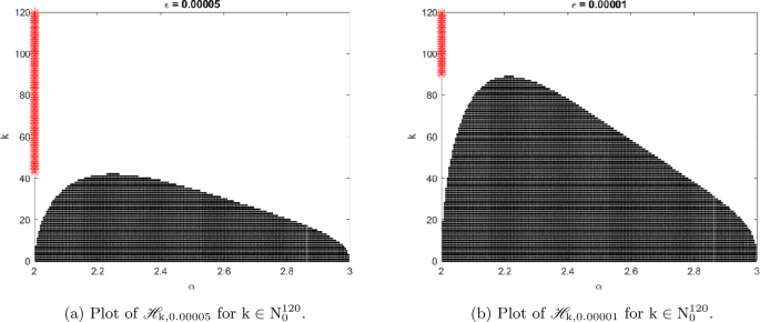

  

  Plot of $\mathscr{H}_{\mathrm{k},\epsilon }$ for $\mathrm{k}\in \mathrm{N}_{0}^{120}$ and different values of ϵ

• In Fig. 2, the set $\mathscr{H}_{\mathrm{k},0.000005}$ in Fig. 2(a) and the set $\mathscr{H}_{\mathrm{k},0.000001}$ in Fig. 2(b) have the same values of k in $\mathrm{N}_{0}^{120}$. In Fig. 2(a), we observe that $\mathscr{H}_{\mathrm{k},\epsilon }=\emptyset$ for $\mathrm{k}\geqq 120$, whereas $\mathscr{H}_{\mathrm{k},\epsilon }=\emptyset$ for $\mathrm{k}\geqq 165$ in Fig. 2(b).

  Figure 2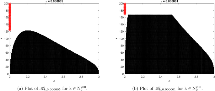

  

  Plot of $\mathscr{H}_{\mathrm{k},\epsilon }$ for $\mathrm{k}\in \mathrm{N}_{0}^{200}$ and different values of ϵ

Figure 3

Plot of $\mathscr{M}_{\mathrm{k},\epsilon }$ for $\mathrm{k}\in \mathrm{N}_{0}^{200}$ and different values of ϵ

Figure 4

Plot of $\mathscr{M}_{\mathrm{k},\epsilon }$ for $\mathrm{k}\in \mathrm{N}_{0}^{250}$ and different values of ϵ

In both Figs. 1 and 2, the set $\mathscr{H}_{\mathrm{k},\epsilon }$ remains empty for less values of k when ϵ is larger than when ϵ is small. Furthermore, this set arises to be enriched almost surely toward α values closer to 2 than those closer to 3; especially, for $\alpha \approx 2.2$, it appears that the set $\mathscr{H}_{\mathrm{k},\epsilon }$ is most concentrated.

Next, we consider the set $\mathscr{M}_{\mathrm{k},\epsilon }$ for various values of k and ϵ:

• Considering Fig. 3, we see that the set $\mathscr{M}_{\mathrm{k},0.0005}$ in Fig. 3(a) and the set $\mathscr{M}_{\mathrm{k},0.0001}$ in Fig. 3(b) have the same values of k in $\mathrm{N}_{0}^{200}$. Moreover, in Fig. 3(a), we can observe that $\mathscr{M}_{\mathrm{k},\epsilon }=\emptyset$ for $\mathrm{k}\geqq 130$, whereas $\mathscr{M}_{\mathrm{k},\epsilon }=\emptyset$ for $\mathrm{k}\geqq 165$ in Fig. 3(b) for a smaller value of ϵ.

• Considering Fig. 4, we note that the set $\mathscr{M}_{\mathrm{k},0.00005}$ in Fig. 4(a) and the set $\mathscr{M}_{\mathrm{k},0.00001}$ in Fig. 4(b) have the same values of k in $\mathrm{N}_{0}^{200}$. Furthermore, in Figs. 4(a) and 4(b), we can note that $\mathscr{M}_{\mathrm{k},\epsilon }=\emptyset$ for $\mathrm{k}\geqq 170$.

Just like in Figs. 1 and 2, we can conclude that in both Figs. 3 and 4, the set $\mathscr{M}_{\mathrm{k},\epsilon }$ tends to remain empty for less values of k when ϵ is larger than when ϵ is small.

Finally, from the sets $\mathscr{H}_{\mathrm{k},\epsilon }$ and $\mathscr{M}_{\mathrm{k},\epsilon }$ we can conclude that:

• Both sets $\mathscr{H}_{\mathrm{k},\epsilon }$ and $\mathscr{M}_{\mathrm{k},\epsilon }$ tend to remain empty for less values of k when ϵ is larger than when ϵ is small.

• The set $\mathscr{H}_{\mathrm{k},\epsilon }$ gives a larger empty space even for ϵ smaller than the set of $\mathscr{M}_{\mathrm{k},\epsilon }$, which has large nonempty space values.

• Theorems 3.2 and 3.3 may be employed for the largest number of time steps whenever α approaches 2.2 and $0 < \epsilon \ll 1$.

5 Conclusions

We have performed analytical and numerical convexity analysis for discrete delta Riemann–Liouville fractional difference operators. The numerical part can be summarized as follows:

• An alternative definition for the discrete delta Riemann–Liouville fractional difference is derived in Theorem 2.1.

• A $\Delta ^{2}$ formula is obtained in Lemma 3.1.

• A relationship between the positivity of $({}^{\mathrm{RL}}_{w_{0}}\Delta ^{\alpha} \mathrm{f} )( \mathrm{t})$ and convexity of f is considered in Theorem 3.1.

• Two sets $\mathscr{H}_{\mathrm{k},\epsilon}$ and $\mathscr{M}_{\mathrm{k},\epsilon}$ are defined based on the basic lemmas, and it is shown that they are decreasing in Lemma 3.2.

• Based on the decrease of these sets, relationships between the negative lower bound of $({}^{\mathrm{RL}}_{w_{0}}\Delta ^{\alpha} \mathrm{f} )( \mathrm{t})$ and convexity of f has been derived in Theorems 3.2 and 3.3 on a finite time set $\mathrm{N}_{w_{0}}^{\mathrm{P}}$.

On the other hand, the numerical part in Sect. 4 can be summarized as follows:

• The domain of solutions of the sets $\mathscr{H}_{\mathrm{k},\epsilon}$ and $\mathscr{M}_{\mathrm{k},\epsilon}$ for various values of k and ϵ has been illustrated in Figs. 1–4.

• In view of these figures, the validity and applicability of Theorems 3.2 and 3.3 is explained.

• We have concluded that when ϵ is small, the sets $\mathscr{H}_{\mathrm{k},\epsilon}$ and $\mathscr{M}_{\mathrm{k},\epsilon}$ tend to remain nonempty for more values of k than for larger ϵ. Furthermore, the sets appear to be enriched powerfully toward the values of α closer to 2 than those closer to 3 for all values of ϵ.

References

Kilbas, A.A., Srivastava, H.M., Trujillo, J.J.: Theory and Applications of Fractional Differential Equations. Elsevier, Amsterdam (2006)
Srivastava, H.M.: Fractional-order derivatives and integrals: introductory overview and recent developments. Kyungpook Math. J. 60, 73–116 (2020)
Srivastava, H.M.: Some parametric and argument variations of the operators of fractional calculus and related special functions and integral transformations. J. Nonlinear Convex Anal. 22, 1501–1520 (2021)
Srivastava, H.M.: An introductory overview of fractional-calculus operators based upon the Fox–Wright and related higher transcendental functions. J. Adv. Eng. Comput. 5, 135–166 (2021)
Goodrich, C.S., Peterson, A.C.: Discrete Fractional Calculus. Springer, Berlin (2015)
Atici, F.M., Eloe, P.W.: Discrete fractional calculus with the nabla operator. Electron. J. Qual. Theory Differ. Equ. 2009, 3 (2009)
Atici, F.M., Sengül, S.: Modeling with fractional difference equations. J. Math. Anal. Appl. 369, 1–9 (2010)
Atici, F.M., Atici, M., Belcher, M., Marshall, D.: A new approach for modeling with discrete fractional equations. Fundam. Inform. 151, 313–324 (2017)
Atici, F., Sengul, S.: Modeling with discrete fractional equations. J. Math. Anal. Appl. 369, 1–9 (2010)
Goodrich, C.S.: On discrete sequential fractional boundary value problems. J. Math. Anal. Appl. 385, 111–124 (2012)
Chen, C.R., Bohner, M., Jia, B.G.: Ulam–Hyers stability of Caputo fractional difference equations. Math. Methods Appl. Sci. 42, 7461–7470 (2019)
Abdeljawad, T.: On delta and nabla Caputo fractional differences and dual identities. Discrete Dyn. Nat. Soc. 2013, Article ID 406910 (2013)
Lizama, C.: The Poisson distribution, abstract fractional difference equations, and stability. Proc. Am. Math. Soc. 145, 3809–3827 (2017)
Srivastava, H.M., Mohammed, P.O., Ryoo, C.S., Hamed, Y.S.: Existence and uniqueness of a class of uncertain Liouville–Caputo fractional difference equations. J. King Saud Univ., Sci. 33, 101497 (2021)
Lu, Q., Zhu, Y.: Comparison theorems and distributions of solutions to uncertain fractional difference equations. J. Comput. Appl. Math. 376, 112884 (2020)
Atici, F.M., Eloe, P.W.: A transform method in discrete fractional calculus. Int. J. Differ. Equ. 2, 165–176 (2007)
Mohammed, P.O., Abdeljawad, T.: Discrete generalized fractional operators defined using h-discrete Mittag-Leffler kernels and applications to AB fractional difference systems. Math. Methods Appl. Sci., 1–26 (2020). https://doi.org/10.1002/mma.7083
Atici, F.M., Atici, M., Nguyen, N., Zhoroev, T., Koch, G.: A study on discrete and discrete fractional pharmaco kinetics pharmaco dynamics models for tumor growth and anti-cancer effects. Comput. Math. Biophys. 7, 10–24 (2019)
Silem, A., Wu, H., Zhang, D.-J.: Discrete rogue waves and blow-up from solitons of a nonisospectral semi-discrete nonlinear Schrödinger equation. Appl. Math. Lett. 116, 107049 (2021)
Ferreira, R.A.C., Torres, D.F.M.: Fractional h-difference equations arising from the calculus of variations. Appl. Anal. Discrete Math. 5, 110–121 (2011)
Wu, G., Baleanu, D.: Discrete chaos in fractional delayed logistic maps. Nonlinear Dyn. 80, 1697–1703 (2015)
He, J.W., Zhang, L., Zhou, Y., Ahmad, B.: Existence of solutions for fractional difference equations via topological degree methods. Adv. Differ. Equ. 2018, 153 (2018)
Goodrich, C.S., Lyons, B.: Positivity and monotonicity results for triple sequential fractional differences via convolution. Analysis 40, 89–103 (2020)
Goodrich, C.S., Lizama, C.: Positivity, monotonicity, and convexity for convolution operators. Discrete Contin. Dyn. Syst. 40, 4961–4983 (2020)
Mohammed, P.O., Abdeljawad, T., Hamasalh, F.K.: On Riemann–Liouville and Caputo fractional forward difference monotonicity analysis. Mathematics 9, 1303 (2021)
Mohammed, P.O., Srivastava, H.M., Baleanu, D., Elattar, E.E., Hamed, Y.S.: Positivity analysis for the discrete delta fractional differences of the Riemann–Liouville and Liouville–Caputo types. Electron. Res. Arch. 30, 3058–3070 (2022)
Nonlaopon, K., Mohammed, P.O., Hamed, Y.S., Muhammad, R.S., Brzo, A.B., Aydi, H.: Analytical and numerical monotonicity analyses for discrete delta fractional operators. Mathematics 10, 1753 (2022)
Dahal, R., Goodrich, C.S.: Theoretical and numerical analysis of monotonicity results for fractional difference operators. Appl. Math. Lett. 117, 107104 (2021)
Atici, F., Uyanik, M.: Analysis of discrete fractional operators. Appl. Anal. Discrete Math. 9, 139–149 (2015)
Dahal, R., Goodrich, C.S.: Analysis of convexity results for discrete fractional nabla operators. Rocky Mt. J. Math. 51, 1981–2001 (2021)
Erbe, L., Goodrich, C.S., Jia, B., Peterson, A.C.: Survey of the qualitative properties of fractional difference operators: monotonicity, convexity, and asymptotic behavior of solutions. Adv. Differ. Equ. 2016, 43 (2016)
Mohammed, P.O., Almutairi, O., Agarwal, R.P., Hamed, Y.S.: On convexity, monotonicity and positivity analysis for discrete fractional operators defined using exponential kernels. Fractal Fract. 6, 55 (2022)
Abdeljawad, T., Atici, F.: On the definitions of nabla fractional operators. Abstr. Appl. Anal. 2012, Article ID 406757 (2012)
Abdeljawad, T.: Different type kernel h-fractional differences and their fractional h-sums. Chaos Solitons Fractals 116, 146–156 (2018)
Carlson, B.C.: Special Functions of Applied Mathematics. Academic Press, New York (1977)
Acknowledgements
This work was supported by the Taif University Researchers Supporting Project (No. TURSP-2020/155), Taif University, Taif, Saudi Arabia, and the fifth author would like to thank Prince Sultan University for the support through the TAS research lab.
Funding
Not applicable.
Author information
Authors and Affiliations
Contributions
Conceptualization, P.O.M., H.M.S., D.B., E.A.-S. and T.A.; Data curation, P.O.M., H.M.S., D.B. and T.A.; Formal analysis, H.M.S., D.B. and T.A.; Funding acquisition, D.B., E.A.-S. and Y.S.H.; Investigation, H.M.S., P.O.M., D.B., E.A.-S., T.A. and Y.S.H.; Methodology, E.A.-S., T.A. and Y.S.H.; Project administration, D.B., E.A.-S. and H.M.S.; Resources, P.O.M. and Y.S.H.; Software, H.M.S.; Supervision, D.B., H.M.S., E.A.-S. and T.A.; Validation, P.O.M., D.B., T.A.; Visualization, T.A.; Writing – original draft, P.O.M. and H.M.S.; Writing – review & editing, D.B., Y.S.H. and T.A. All authors have read and agreed to the published version of the manuscript.
Corresponding authors
Ethics declarations
Competing interests
The authors declare no competing interests.
Rights and permissions
Open Access This article is licensed under a Creative Commons Attribution 4.0 International License, which permits use, sharing, adaptation, distribution and reproduction in any medium or format, as long as you give appropriate credit to the original author(s) and the source, provide a link to the Creative Commons licence, and indicate if changes were made. The images or other third party material in this article are included in the article’s Creative Commons licence, unless indicated otherwise in a credit line to the material. If material is not included in the article’s Creative Commons licence and your intended use is not permitted by statutory regulation or exceeds the permitted use, you will need to obtain permission directly from the copyright holder. To view a copy of this licence, visit http://creativecommons.org/licenses/by/4.0/.
About this article
Cite this article
Baleanu, D., Mohammed, P.O., Srivastava, H.M. et al. On convexity analysis for discrete delta Riemann–Liouville fractional differences analytically and numerically. J Inequal Appl 2023, 4 (2023). https://doi.org/10.1186/s13660-023-02916-2
Received:
Accepted:
Published:
DOI: https://doi.org/10.1186/s13660-023-02916-2