Adapting step size algorithms for solving split equilibrium problems with applications to signal recovery

Abstract

Recent developments in split equilibrium problems (SEPs) have found practical applications in convex optimization problems, information theory, and signal processing. In this paper, we present three novel algorithms with no prior knowledge of the operator norm of a bounded linear operator to approximated solutions for SEPs. Strong convergence results are well presented under appropriate conditions. In addition, we illustrate our main results by providing various numerical examples. Their computational performances are compared with those previously studied in the literature, and the results are presented by showing numerical implementation of the sparse sensor signal recovery problem.

1 Introduction

Throughout this work, let two nonempty closed convex subsets C and D be in two real Hilbert spaces $H_{1}$ and $H_{2}$, respectively. This paper focuses on the split equilibrium problems (SEPs) introduced by He [1], which are used to solve a point $w^{*}\in C$ that

$$\begin{aligned} f \bigl(w^{*},p \bigr)\geq 0, \quad\forall p\in C, \end{aligned}$$

(1)

and a point $v^{*}=Aw^{*}\in D$ solves

$$\begin{aligned} g \bigl(v^{*},q \bigr)\geq 0, \quad\forall q\in D, \end{aligned}$$

(2)

where f and g are nonlinear bi-functions on $C\times C$ and $D\times D$, respectively, and an operator $A:H_{1}\to H_{2}$ is bounded linear with its adjoint operator $A^{*}$. The equilibrium problem plays a vital role in various branches of science, optimization, and economics (see [2–6] for details). We provide a set of all solutions for the split equilibrium problems (SEPs) (1)–(2) as follows:

$$\begin{aligned} \Omega _{\mathrm{SEP}s}= \bigl\{ u\in \mathrm{EP}(f) : Au\in \mathrm{EP}(g) \bigr\} , \end{aligned}$$

(3)

where $\mathrm{EP}(f)$ and $\mathrm{EP}(g)$ denote the solution sets of classical equilibrium problems (1) and (2), respectively.

Over a decade, many methods have been constructed and developed to find solutions for SEPs (1)–(2). The development of algorithms to solve the SEPs is stated as follows. Kazmi and Rizvi [7], in 2013, devised an iterative technique to examine a solution for the SEPs. Let a real number $L_{A}$ be the spectral radius of $A^{*}A$, $P_{C}$ be an orthogonal projection onto C, and a map $E:C\to H_{1}$ be α-inverse strongly monotone. Their algorithm was defined as follows:

$$\begin{aligned} \textstyle\begin{cases} w_{1}\in H_{1}, \quad \forall n\geq 1, \\ v_{n}=T_{r_{n}}^{f}(I+\gamma A^{*}(T_{r_{n}}^{g}-I)A)w_{n}, \\ u_{n}=P_{C}(I-\lambda _{n} E)v_{n}, \\ w_{n+1}=\mu _{n} u+\rho _{n} w_{n}+\sigma _{n} Wu_{n}, \end{cases}\displaystyle \end{aligned}$$

(4)

where $\gamma \in (0,\frac{1}{L_{A}})$, $r_{n} >0$, $\lambda _{n}\in (2,2\alpha )$, and real sequences $\{\mu _{n} \}, \{\rho _{n} \}$, and $\{\sigma _{n} \}$ are in $(0,1)$. Under suitable conditions of all parameters, the iterative method (4) provided the strong convergence for the SEPs.

In 2016, Suantai [8] presented an iterative algorithm for solving the SEPs as follows:

$$\begin{aligned} \textstyle\begin{cases} x_{1}\in C, \quad \forall n\geq 1, \\ u_{n}=T_{r_{n}}^{f}(I+\gamma A^{*}(T_{r_{n}}^{g}-I)A)x_{n}, \\ x_{n+1}\in \mu _{n} x_{n} + (1-\mu _{n})Wu_{n}, \end{cases}\displaystyle \end{aligned}$$

(5)

where W is a $\frac{1}{2}$-nonspreading multivalued mapping, $\gamma \in (0,\frac{1}{L_{A}})$, $\{r_{n}\}\subseteq (0,\infty )$, and $\{\mu _{n} \}\subseteq (0,1)$. Suantai also provided a weak convergence result.

By using Suantai’s ideas, Onjai-uea and Phuengrattana [9] constructed and developed an algorithm to solve the SEPs in 2017 as follows:

$$\begin{aligned} \textstyle\begin{cases} x_{1}\in C, \quad \forall n\geq 1, \\ u_{n}=T_{r_{n}}^{f}(I+\gamma A^{*}(T_{r_{n}}^{g}-I)A)x_{n}, \\ y_{n}\in \alpha _{n} x_{n} + (1-\alpha _{n})Wu_{n}, \\ x_{n+1}\in \mu _{n} x_{n} + (1-\mu _{n})Wy_{n}, \end{cases}\displaystyle \end{aligned}$$

(6)

where W is a multivalued λ-hybrid mapping, $\gamma \in (0,\frac{1}{L_{A}})$, $\{r_{n}\}\subseteq (0,\infty )$, and $\{\alpha _{n} \} , \{\mu _{n} \} \subseteq (0,1)$. Under some appropriate conditions, Onjai-uea and Phuengrattana presented that algorithm (6) weakly converges to a solution for the SEPs. There are many methods to solve the SEPs that are not mentioned above. The reader can refer to [1, 10–12] for details.

Note that the iterative methods (4), (5), and (6) are usually used with the stepsize γ that depends on the operator norm $\|A\|$. Hence this paper is focused on overcoming this difficulty by constructing algorithms with no prior knowledge of operator norm $\|A\|$. For more details about these ideas, the reader is directed to [13, 14]. For any $r_{n}>0$, we define

$$\begin{aligned} &\psi (x):=\frac{1}{2} \bigl\Vert \bigl(I-T_{r_{n}}^{f} \bigr)x \bigr\Vert ^{2}; \end{aligned}$$

(7)

$$\begin{aligned} &\omega (x):=\frac{1}{2} \bigl\Vert \bigl(I-T_{r_{n}}^{g} \bigr)Ax \bigr\Vert ^{2}. \end{aligned}$$

(8)

Consider in case that f and g are indicator functions for the closed convex subsets C and Q of Hilbert spaces, then $T_{r_{n}}^{f}=P_{C}$ and $T_{r_{n}}^{g}=P_{Q}$. Recall that the squared distance functions $\|x-P_{C}x\|^{2}$ and $\|x-P_{Q}x\|^{2}$ are differentiable, we have the gradients ∇ψ and ∇ω of operators ω and ψ, respectively, as follows:

$$\begin{aligned} &\nabla \psi (x):= \bigl(I-T_{r_{n}}^{f} \bigr)x; \end{aligned}$$

(9)

$$\begin{aligned} &\nabla \omega (x):=A^{*} \bigl(I-T_{r_{n}}^{g} \bigr)Ax. \end{aligned}$$

(10)

However, gradients (9) and (10) are not true in general.

By using operators (8)–(9), we construct a new step size by using self-adaptive method to avoid computing the operator norm $\|A\|$ as follows:

$$\begin{aligned} \tau _{n}:= \textstyle\begin{cases} \frac {\rho _{n}\omega (u_{n})}{ \Vert \nabla \omega (u_{n}) \Vert ^{2}+ \Vert \nabla \psi (u_{n}) \Vert ^{2}} & \Vert \nabla \omega (u_{n}) \Vert ^{2}+ \Vert \nabla \psi (u_{n}) \Vert ^{2}\neq 0, \\ 0 &\text{otherwise}, \end{cases}\displaystyle \end{aligned}$$

(11)

where $0<\rho _{n}<4$.

Inspired by the above works, the aims of this papers are as follows: (1) To construct and propose three modified step size algorithms by using new self-adaptive techniques; (2) to obtain theoretical results of strong convergence for the SEPs based on the proposed algorithms; (3) to show the performance of our proposed algorithms by comparing them to the previously developed algorithms by Kazmi and Rizvi [7], Suantai [8], Onjai-uea and Phuengrattana [9]; and (4) to demonstrate the presented results by showing numerical implementation of the sparse sensor signal recovery problem.

The remainder of this paper is organized as follows. Section 2 establishes preliminaries used in this work, and related definitions and lemma are presented. Section 3 introduces the proposed step size algorithms for solving the SEPs with three modifications, and the main theorems are proved. Section 4 then demonstrates the numerical examples of the proposed algorithms and shows theoretical applications in split feasibility problem and optimization problem. Section 5 then gives conclusions of this work.

2 Preliminaries

In this section, we give a preliminary result that is necessary for our consequent analysis. In the weak topology, the set of all limit points is given by $\omega _{w}(u_{n})$ for a sequence $\{u_{n}\}$ in a real Hilbert space. Let $f:C\times C\to \mathbb{R}$ and $g:D\times D\to \mathbb{R}$ be nonlinear bi-functions. Suppose the following assumptions for a bi-function f:

• (A1) $f(s,s)\geq 0$;

• (A2) $f(s,t)+f(t,s)\leq 0$ (f is monotone);

• (A3) $\limsup_{\zeta \to 0} f(\zeta s+(1-\zeta )t,w)\leq f(t,w)$;

• (A4) $s\mapsto f(t,s)$ is a lower semicontinuous and convex function;

for all $s,t,w\in C$. Let $T_{r}^{f}:H_{1}\to C$ be a mapping given by

$$\begin{aligned} T_{r}^{f}(w)= \biggl\lbrace s\in C:f(s,t)+ \frac {1}{r}\langle t-s,s-w \rangle \geq 0, \forall t\in C \biggr\rbrace \end{aligned}$$

(12)

for $r>0$ and for all $w\in H_{1}$.

Definition 2.1

For any $v,w \in C$, the mapping $S: C\to H_{1}$ is said to be

• 1. monotone if $\langle v-w, Sv-Sw \rangle \geq 0$;

• 2. ϑ-inverse strongly monotone (for short ϑ-ism) if $\langle w-v, Sw-Sv \rangle \geq \vartheta \|Sw-Sv\|^{2} \text{ for some } \vartheta > 0$;

• 3. L-Lipschitz continuous if $\|Sw-Sv\|\leq L\|w-v\| \text{ for some } L\in [0,1)$;

• 4. nonexpansive if $\|Sw-Sv\|\leq \|w-v\|$;

• 5. firmly nonexpansive if $\|Sw-Sv\|^{2}\leq \langle Sw-Sv, w-v\rangle$.

Recall that every nonexpansive mapping S satisfies the following inequalities:

• 1. $\langle (v-Sv)-(w-Sw),Sw-Sv\rangle \leq \frac{1}{2}\|(Sv-v)-(Sw-w)\|^{2}$;

• 2. $\langle v-Sv,w-Sv\rangle \leq \frac{1}{2}\|Sv-v\|^{2}$.

Lemma 2.2

For any $v, w\in H_{1}$ and $\theta \in [0,1]$, the following relationships hold:

• 1. $\|w+u\|^{2}\leq \|w\|+2\langle u,w+u \rangle$;

• 2. $\|w-u\|^{2}=\|w\|^{2}+\|u\|^{2}-2\langle w-u,u \rangle$;

• 3. $\|\theta w+(1-\theta )u\|^{2}=\theta \|w\|^{2}+(1-\theta )\|u\|^{2}- \theta (1-\theta )\|w-u\|^{2}$.

Lemma 2.3

For the metric projection $P_{C}$, the following relationships hold:

• 1. $P_{C}$ is a nonexpansive mapping;

• 2. $\|P_{C}v-P_{C}w\|^{2}\leq \langle v-w, P_{C}v-P_{C}w \rangle$;

• 3. $\langle v-P_{C}v, w-P_{C}w\rangle \leq 0$;

• 4. $\|v-P_{C}v\|^{2}+\|w-P_{C}v\|^{2}\leq \|v-w\|^{2}$;

• 5. $\|v-w\|^{2}-\|P_{C}v-P_{C}w\|^{2}\leq \|(v-w)-(P_{C}v-P_{C}w)\|^{2}$;

for any $v, w\in H_{1}$.

Lemma 2.4

([3])

Assume that a bi-function f satisfies assumptions (A1)–(A4) and the mapping $T_{r}^{f}$ is defined by equation (12). Then:

• 1. $T_{r}^{f}$ is nonempty, single-valued, and firmly nonexpansive;

• 2. $\mathrm{EP}(f) = \mathrm{Fix}(T_{r}^{f})$;

• 3. $\mathrm{EP}(f)$ is a closed convex set.

Moreover, see in [15], the mapping $T_{r}^{f}$ satisfies the following inequality:

$$\begin{aligned} \bigl\Vert T_{s}^{f}v-T_{r}^{f}w \bigr\Vert \leq \Vert v-w \Vert + \biggl\vert \frac{s-r}{s} \biggr\vert \bigl\Vert T_{s}^{f}w-w \bigr\Vert \end{aligned}$$

(13)

for any $v,w\in H_{1}$ and $r,s>0$.

Lemma 2.5

([16])

Let $\{w_{n}\}$ and $\{v_{n}\}$ be two bounded sequences and a real sequence $\{\zeta _{n}\} \subseteq [0,1]$ such that

$$\begin{aligned} w_{n+1}=(1-\zeta _{n})v_{n}+\zeta _{n} w_{n}, \quad\forall n\geq 1. \end{aligned}$$

If the following statements hold:

• 1. $\limsup_{n\to \infty}(\|v_{n+1}-v_{n}\|-\|w_{n+1}-w_{n}\|)\leq 0$;

• 2. $0<\liminf_{n\to \infty}\zeta _{n}\leq \limsup_{n\to \infty}\zeta _{n}<1$.

Then $\lim_{n\to \infty}\|v_{n}-w_{n}\|=0$.

Lemma 2.6

([17])

The Hilbert space H satisfies the Opial condition, if $w_{n}\rightharpoonup w$ for any sequence $\{w_{n}\} \in H$ and element $v\in H$ with $v\neq w$, then

$$\begin{aligned} \liminf_{n\to \infty} \Vert w_{n}-w \Vert < \liminf _{n\to \infty} \Vert w_{n}-v \Vert . \end{aligned}$$

Lemma 2.7

([18])

Let $\{w_{n}\} \subseteq (0 , \infty )$ be a sequence of real numbers with

$$\begin{aligned} w_{n+1}\leq (1-\mu _{n})w_{n}+\mu _{n} \delta _{n}+\xi _{n} \end{aligned}$$

for all $n\geq 1$, where

• 1. $\{\mu _{n}\}\subset [0,1]$ and $\sum \mu _{n}=\infty$,

• 2. $\limsup \delta _{n}\leq 0$,

• 3. $\xi _{n}\geq 0$ and $\sum \xi _{n}<\infty$.

Then $\lim_{n\to \infty}w_{n}=0$.

Lemma 2.8

([19])

Suppose that a real number sequence $\{\Gamma _{m}\}$ does not decrease at infinity. This means that there is $\{\Gamma _{m_{i}}\} \subseteq \{\Gamma _{m}\}$ with $\{\Gamma _{m_{i}}\}<\{\Gamma _{m_{i}+1}\}$ $\forall i\geq 0$. Let a sequence of integers $\{\sigma (m)\}_{m\geq m_{0}}$ be given by

$$\begin{aligned} \sigma (m)=\max \{l\leq m : \Gamma _{l}\leq \Gamma _{l+1} \}. \end{aligned}$$

Thus $\{\sigma (m)\}_{m\geq m_{0}}$ is a nondecreasing sequence that verifies $\lim_{m\to \infty}\sigma (m)=\infty$,

$$\begin{aligned} \max \{\Gamma _{\sigma (m)},\Gamma _{m} \}\leq \Gamma _{\sigma (m)+1} \end{aligned}$$

for all $m\geq m_{0}$.

Lemma 2.9

Assume that $\psi :H_1\to \mathbb{R}$ and $\omega :H_2\to \mathbb{R}$ are two functions given by equations (7) and (8), respectively. Then the gradients ∇ω and ∇ψ of the functions ω and ψ are Lipschitz continuous.

Proof

Since $\nabla \omega (p)=A^{*}(I-T_{r_{n}}^{g})Ap$, we have

$$\begin{aligned} & \bigl\Vert \nabla \omega (p)-\nabla \omega (q) \bigr\Vert ^{2} \\ &\quad= \bigl\langle A^{*} \bigl( \bigl(I-T_{r_{n}}^{g} \bigr)Ap- \bigl(I-T_{r_{n}}^{g} \bigr)Aq \bigr),A^{*}( \bigl(I-T_{r_{n}}^{g} \bigr)Ap- \bigl(I-T_{r_{n}}^{g} \bigr)Aq \bigr\rangle \\ &\quad= \bigl\langle \bigl(I-T_{r_{n}}^{g} \bigr)Ap- \bigl(I-T_{r_{n}}^{g} \bigr)Aq,AA^{*}( \bigl(I-T_{r_{n}}^{g} \bigr)Ap- \bigl(I-T_{r_{n}}^{g} \bigr)Aq \bigr\rangle \\ &\quad\leq L_{A} \bigl\Vert \bigl(I-T_{r_{n}}^{g} \bigr)Ap- \bigl(I-T_{r_{n}}^{g} \bigr)Aq \bigr\Vert ^{2}, \end{aligned}$$

(14)

where $L_{A}=\|A\|^{2}$. On the other hand,

$$\begin{aligned} \bigl\langle \nabla \omega (p)-\nabla \omega (q), p-q \bigr\rangle &= \bigl\langle A^{*} \bigl( \bigl(I-T_{r_{n}}^{g} \bigr)Ap- \bigl(I-T_{r_{n}}^{g} \bigr)Aq \bigr),p-q \bigr\rangle \\ &= \bigl\langle \bigl(I-T_{r_{n}}^{g} \bigr)Ap- \bigl(I-T_{r_{n}}^{g} \bigr)Aq,A(p-q) \bigr\rangle \\ &\geq \bigl\Vert \bigl(I-T_{r_{n}}^{g} \bigr)Ap- \bigl(I-T_{r_{n}}^{g} \bigr)Aq \bigr\Vert ^{2}. \end{aligned}$$

(15)

By combining (14) with (15), we get that

$$\begin{aligned} \bigl\langle \nabla \omega (p)-\nabla \omega (q), p-q \bigr\rangle \geq \frac {1}{L_{A}} \bigl\Vert \nabla \omega (p)-\nabla \omega (q) \bigr\Vert ^{2} . \end{aligned}$$

Thus ∇ω is $\frac{1}{L_{A}}$-inverse strongly monotone. Moreover,

$$\begin{aligned} \bigl\langle \nabla \omega (p)-\nabla \omega (q),p-q \bigr\rangle \leq \Vert p-q \Vert \bigl\Vert \nabla \omega (p)-\nabla \omega (q) \bigr\Vert . \end{aligned}$$

Hence $\|\nabla \omega (p)-\nabla \omega (q)\|\leq L_{A}\|p-q\|$. Similarly, ∇ψ is Lipschitz continuous. □

3 Results

This section presents and analyzes our three iterative algorithms generated sequences that strongly converge to a solution of SEPs (1)–(2) and the fixed point problems of a nonexpansive mapping. In the sequel, the solution set is given by

$$\begin{aligned} \Psi =\Omega _{\mathrm{SEP}s}\cap \mathrm{Fix}(S). \end{aligned}$$

(16)

Before starting the results, assume that two bi-functions f and g satisfy assumptions (A1)–(A4) and g is upper semicontinuous. Let a mapping S be nonexpansive on C and $\Psi \neq \emptyset$. Now, we constructed and then analyzed three algorithms as follows.

Condition 3.1

Suppose that $\{r_{n}\}\subseteq (0,\infty )$, a is a constant, $\{\rho _{n} \}$ is any positive sequence, and real parameter sequences $\{\alpha _{n} \}, \{\beta _{n} \}, \{\gamma _{n} \}$, and $\{\kappa _{n} \}$ satisfy $\alpha _{n}, \beta _{n}, \gamma _{n}, \kappa _{n} \in (0, 1)$, and the following conditions hold:

• (C1) $\alpha _{n}+\beta _{n}+\gamma _{n}=1$;

• (C2) $\sum_{n=0}^{\infty}\alpha _{n}=\infty , \lim_{n\to \infty}\alpha _{n}=0$;

• (C3) $\lim_{n\to \infty}\kappa _{n}=0 \textit{ and } \lim_{n\to \infty} \frac{\kappa _{n}}{\alpha _{n}}=0$;

• (C4) $\lim_{n\to \infty}|r_{n+1}-r_{n}|=0 \textit{ and } 0< a\leq r_{n}$;

• (C5) $0<\lim \inf_{n\to \infty}\beta _{n}\leq \lim \sup_{n\to \infty} \beta _{n}<1$;

• (C6) $\lim_{n\to \infty} ( \frac {\gamma _{n+1}}{1-\beta _{n+1}}- \frac {\gamma _{n}}{1-\beta _{n}} ) =0$;

• (C7) $\inf \rho _{n}(4-\rho _{n})>0$ and $0<\rho _{n}<4$.

Theorem 3.1

The sequence $\{x_{n}\}$ generated by Algorithm 1 converges strongly to a solution $s\in \Psi$, where $s=P_{\Psi }u$.

Algorithm 1

The first algorithm to solve split equilibrium problems

Proof

Since Ψ is a nonempty set, take each $c\in \Psi$, this implies $c=T_{r_{n}}^{f}(c)$ and $Ac=T_{r_{n}}^{g}(Ac)$. Thus $(I-T_{r_{n}}^{g})Ac=Ac-Ac=0$. Since $\nabla \omega (x_{n})=A^{*}(T_{r_{n}}^{g}-I)Ax_{n}$ and $T_{r_{n}}^{g}-I$ is a firmly nonexpansive mapping, we find that

$$\begin{aligned} \bigl\langle \nabla \omega (x_{n}),x_{n}-c \bigr\rangle &= \bigl\langle A^{*} \bigl(T_{r_{n}}^{g}-I \bigr)Ax_{n}, x_{n}-c \bigr\rangle \\ &= \bigl\langle \bigl(T_{r_{n}}^{g}-I \bigr)Ax_{n}- \bigl(T_{r_{n}}^{g}-I \bigr)As,Ax_{n}-Ac \bigr\rangle \\ &\geq \bigl\Vert \bigl(T_{r_{n}}^{g}-I \bigr)Ax_{n} \bigr\Vert ^{2} \\ &=2\omega (x_{n}). \end{aligned}$$

(17)

By using the fact that $T_{r_{n}}^{f}(I+\tau _{n}A^{*}(T_{r_{n}}^{g}-I)A)$ is a nonexpansive mapping, we can easily verify that

$$\begin{aligned} \Vert u_{n}-c \Vert ^{2}={}& \bigl\Vert T_{r_{n}}^{f} \bigl(I+\tau _{n} A^{*} \bigl(T_{r_{n}}^{g}-I \bigr) A \bigr)x_{n}-T_{r_{n}}^{f}c \bigr\Vert ^{2} \\ \leq {}& \bigl\Vert \bigl(I+\tau _{n} A^{*} \bigl(T_{r_{n}}^{g}-I \bigr) A \bigr)x_{n}-c \bigr\Vert ^{2} \\ ={}& \bigl\Vert x_{n}-\tau _{n}\nabla \omega (x_{n})-c \bigr\Vert ^{2} \\ \leq{} & \Vert x_{n}-c \Vert ^{2}+\tau _{n}^{2} \bigl\Vert \nabla \omega (x_{n}) \bigr\Vert ^{2}-2 \tau _{n} \bigl\langle x_{n}-c, \nabla \omega (x_{n}) \bigr\rangle \\ \leq {}& \Vert x_{n}-c \Vert ^{2}+\tau _{n}^{2} \bigl\Vert \nabla \omega (x_{n}) \bigr\Vert ^{2}-4 \tau _{n} \omega (x_{n}) \\ ={}& \Vert x_{n}-c \Vert ^{2}+ \frac{\rho ^{2}_{n}\omega ^{2}(x_{n})}{( \Vert \nabla \omega (x_{n}) \Vert ^{2}+ \Vert \nabla \psi (x_{n}) \Vert ^{2})^{2}} \bigl\Vert \nabla \omega (x_{n}) \bigr\Vert ^{2} \\ &{}-4 \frac{\rho _{n}\omega ^{2}(x_{n})}{ \Vert \nabla \omega (x_{n}) \Vert ^{2}+ \Vert \nabla \psi (x_{n}) \Vert ^{2}} \\ \leq{} & \Vert x_{n}-c \Vert ^{2}+ \frac{\rho ^{2}_{n}\omega ^{2}(x_{n})}{ \Vert \nabla \omega (x_{n}) \Vert ^{2}+ \Vert \nabla \psi (x_{n}) \Vert ^{2}} \\ &{}-4 \frac{\rho _{n}\omega ^{2}(x_{n})}{ \Vert \nabla \omega (x_{n}) \Vert ^{2}+ \Vert \nabla \psi (x_{n}) \Vert ^{2}} \\ ={}& \Vert x_{n}-c \Vert ^{2}-\rho _{n}(4-\rho _{n}) \frac {\omega ^{2}(x_{n})}{ \Vert \nabla \omega (x_{n}) \Vert ^{2}+ \Vert \nabla \psi (x_{n}) \Vert ^{2}}. \end{aligned}$$

(18)

This implies that

$$\begin{aligned} \Vert u_{n}-c \Vert \leq \Vert x_{n}-c \Vert . \end{aligned}$$

(19)

Now, let $v\in C$ be fixed and $y_{n}=\kappa _{n} v+(1-\kappa _{n})u_{n}$. We find that

$$\begin{aligned} \Vert y_{n}-c \Vert &= \bigl\Vert \kappa _{n} v+(1-\kappa _{n})u_{n}-c \bigr\Vert \\ &\leq (1-\kappa _{n}) \Vert u_{n}-c \Vert +\kappa _{n} \Vert v-c \Vert \\ &\leq (1-\kappa _{n}) \Vert x_{n}-c \Vert +\kappa _{n} \Vert v-c \Vert . \end{aligned}$$

(20)

Also, we find that

$$\begin{aligned} \Vert y_{n}-c \Vert ^{2}&= \bigl\Vert (1-\kappa _{n}) (u_{n}-c)+\kappa _{n}(v-c) \bigr\Vert ^{2} \\ &\leq (1-\kappa _{n}) \Vert u_{n}-c \Vert ^{2}+2\kappa _{n}\langle v-c,y_{n}-c \rangle . \end{aligned}$$

(21)

By setting $\varrho _{n}=(\alpha _{n}+\kappa _{n}\gamma _{n})$ and using (18) and (20), we obtain

$$\begin{aligned} \Vert x_{n+1}-c \Vert &= \Vert \alpha _{n} u+\beta _{n} x_{n}+\gamma _{n}Sy_{n}-c \Vert \\ &=\beta _{n} \Vert x_{n}-c \Vert + \bigl\Vert \alpha _{n}(u-c)+\gamma (Sy_{n}-c) \bigr\Vert \\ &\leq \beta _{n} \Vert x_{n}-c \Vert +\alpha _{n} \Vert u-c \Vert +\gamma _{n} \Vert y_{n}-c \Vert \\ &\leq \alpha _{n} \Vert u-c \Vert +\beta _{n} \Vert x_{n}-c \Vert +\gamma _{n} \bigl\lbrace \kappa _{n} \Vert v-c \Vert +(1-\kappa _{n}) \Vert x_{n}-c \Vert \bigr\rbrace \\ &=(\beta _{n}+\gamma _{n}-\kappa _{n}\gamma _{n}) \Vert x_{n}-c \Vert +\alpha _{n} \Vert u-c \Vert +\kappa _{n}\gamma _{n} \Vert v-c \Vert \\ &\leq (1-\varrho _{n}) \Vert x_{n}-c \Vert +\varrho _{n}\max \bigl\lbrace \Vert u-c \Vert , \Vert v-c \Vert \bigr\rbrace \\ &\leq\max \bigl\lbrace \Vert x_{n}-c \Vert , \Vert u-c \Vert , \Vert v-c \Vert \bigr\rbrace . \end{aligned}$$

(22)

It concludes that $\{x_{n}\}$ is bounded, and two sequences $\{u_{n}\}$, $\{y_{n} \}$ are also bounded. Because $c=T_{r_{n}}^{f}c$ and $T_{r_{n}}^{f}$ is a firmly nonexpansive mapping, thus

$$\begin{aligned} \Vert u_{n}-c \Vert ^{2}={}& \|T_{r_{n}}^{f} \bigl(x_{n}+\tau _{n}A^{*} \bigl(T_{r_{n}}^{g}-I \bigr)Ax_{n} \bigr))-c \|^{2} \\ \leq {}& \bigl\langle x_{n}+\tau _{n}A^{*} \bigl(T_{r_{n}}^{g}-I \bigr)Ax_{n}-c, u_{n}-c \bigr\rangle \\ ={}&\frac {1}{2} \bigl\lbrace \Vert x_{n}-s \Vert ^{2}- \Vert x_{n}-u_{n} \Vert ^{2}- \tau _{n}^{2} \bigl\Vert \nabla \omega (x_{n}) \bigr\Vert + \Vert u_{n}-c \Vert ^{2} \\ &{}+2\tau _{n} \bigl\langle \nabla \omega (x_{n}), x_{n}-u_{n} \bigr\rangle \bigr\rbrace \\ \leq{} & \Vert x_{n}-c \Vert ^{2}- \Vert x_{n}-u_{n} \Vert ^{2}+2\tau _{n} \Vert x_{n}-u_{n} \Vert \bigl\Vert \nabla \omega (x_{n}) \bigr\Vert . \end{aligned}$$

(23)

Thus, by using inequalities (21) and (23), we get that

$$\begin{aligned} \Vert x_{n+1}-c \Vert ^{2} \leq {}&\beta _{n} \Vert x_{n}-c \Vert ^{2}+\alpha _{n} \Vert u-c \Vert ^{2}+ \gamma _{n} \Vert Sy_{n}-c \Vert ^{2} \\ \leq {}&\beta _{n} \Vert x_{n}-c \Vert ^{2}+ \alpha _{n} \Vert u-c \Vert ^{2}+\kappa _{n} \gamma _{n} \Vert v-c \Vert ^{2}+\gamma _{n}(1- \kappa _{n}) \Vert u_{n}-c \Vert ^{2} \\ \leq {}&\alpha _{n} \Vert u-c \Vert ^{2}+\beta _{n} \Vert x_{n}-c \Vert ^{2}+\kappa _{n} \gamma _{n} \Vert v-c \Vert ^{2} \\ &{}+(\gamma _{n}-\kappa _{n}\gamma _{n}) \bigl\lbrace \Vert x_{n}-c \Vert ^{2}- \Vert x_{n}-u_{n} \Vert ^{2}+2\tau _{n} \Vert x_{n}-u_{n} \Vert \bigl\Vert \nabla \omega (x_{n}) \bigr\Vert \bigr\rbrace \\ \leq {}&\alpha _{n} \Vert u_{n}-c \Vert ^{2}+(1-\alpha _{n}-\kappa _{n}\gamma _{n}) \Vert x_{n}-c \Vert ^{2}+\kappa _{n}\gamma _{n} \Vert v-c \Vert ^{2} \\ &{}+(\kappa _{n}\gamma _{n}-\gamma _{n}) \Vert x_{n}-u_{n} \Vert ^{2}+2\rho _{n} \gamma _{n}(1-\kappa _{n})\omega (x_{n}) \Vert x_{n}-u_{n} \Vert \\ \leq{} &\alpha _{n} \Vert u-c \Vert ^{2}+ \Vert x_{n}-c \Vert ^{2}+\kappa _{n}\gamma _{n} \Vert v-c \Vert ^{2}-(\gamma _{n}+\kappa _{n}\gamma _{n}) \Vert x_{n}-u_{n} \Vert ^{2} \\ &{}+2\rho _{n}(\gamma _{n}-\kappa _{n}\gamma _{n})\omega (x_{n}) \Vert x_{n}-u_{n} \Vert . \end{aligned}$$

(24)

This implies that

$$\begin{aligned} (\gamma _{n}-\kappa _{n}\gamma _{n}) \Vert x_{n}-u_{n} \Vert ^{2} \leq {}& \Vert x_{n}-c \Vert ^{2}+\alpha _{n} \Vert u-c \Vert ^{2}- \Vert x_{n+1}-c \Vert ^{2} \\ &{}+2\rho _{n}(\gamma _{n}-\kappa _{n}\gamma _{n})\omega (x_{n}) \Vert u_{n}-x_{n} \Vert . \end{aligned}$$

(25)

By setting $s=P_{\Psi }u$, we next prove that $\|x_{n+1}-x_{n}\|\to 0$ and $x_{n}\to s$. By using inequality (18), we note that

$$\begin{aligned} \Vert x_{n+1}-s \Vert ^{2}={}& \Vert \alpha _{n} u+\beta _{n} x_{n} +\gamma _{n} Sy_{n}-s \Vert ^{2} \\ \leq {}&\alpha _{n} \Vert u-s \Vert ^{2}+\beta _{n} \Vert x_{n}-s \Vert ^{2}+\kappa _{n} \gamma _{n} \Vert v-s \Vert ^{2}+\gamma _{n}(1-\kappa _{n}) \Vert u_{n}-s \Vert ^{2} \\ \leq{} &\alpha _{n} \Vert u-s \Vert ^{2}+\beta _{n} \Vert x_{n}-s \Vert ^{2}+\kappa _{n} \gamma _{n} \Vert v-s \Vert ^{2}+(\gamma _{n}-\kappa _{n}\gamma _{n}) \biggl[ \Vert x_{n}-s \Vert ^{2} \\ &{}- \bigl(4\rho _{n}-\rho _{n}^{2} \bigr) \frac {\omega ^{2}(x_{n})}{ \Vert \nabla \omega (x_{n}) \Vert ^{2}+ \Vert \nabla \psi (x_{n}) \Vert ^{2}} \biggr] \\ \leq {}&\alpha _{n} \Vert u-s \Vert ^{2}+ \Vert x_{n}-s \Vert ^{2}+\kappa _{n}\gamma _{n} \Vert v-s \Vert ^{2} \\ &{}-\gamma _{n}(1-\kappa _{n}) \bigl(4\rho _{n}- \rho _{n}^{2} \bigr) \frac {\omega ^{2}(x_{n})}{ \Vert \nabla \omega (x_{n}) \Vert ^{2}+ \Vert \nabla \psi (x_{n}) \Vert ^{2}}. \end{aligned}$$

(26)

This implies that

$$\begin{aligned} &\gamma _{n}(1-\kappa _{n})\rho _{n}(4-\rho _{n}) \frac {\omega ^{2}(x_{n})}{ \Vert \nabla \omega (x_{n}) \Vert ^{2}+ \Vert \nabla \psi (x_{n}) \Vert ^{2}} \\ &\quad\leq \Vert x_{n}-s \Vert ^{2}+\alpha _{n} \Vert u-s \Vert ^{2}+\kappa _{n}\gamma _{n} \Vert v-s \Vert ^{2}- \Vert x_{n+1}-s \Vert ^{2}. \end{aligned}$$

(27)

Next, we consider two possible cases to show $\|x_{n}-s\|\to 0$ as $n\to \infty$.

Case 1. Assume that, for existing $n_0\in \mathbb{N}$, a sequence $\{\|x_{n}-s\|^{2} \}$ is nonincreasing. Then the limit of a sequence $\lim_{n\to \infty}\|x_{n}-s\|$ exists and

$$\begin{aligned} \lim_{n\to \infty} \bigl( \Vert x_{n+1}-s \Vert - \Vert x_{n}-s \Vert \bigr)=0. \end{aligned}$$

Since the sequences $\alpha _{n}$ and $\kappa _{n}$ tend to 0, then by using inequality (27), we get that

$$\begin{aligned} \rho _{n}(4-\rho _{n}) \frac {\gamma _{n}\omega ^{2}(x_{n})}{ \Vert \nabla \omega (x_{n}) \Vert ^{2}+ \Vert \nabla \psi (x_{n}) \Vert ^{2}} \to 0. \end{aligned}$$

Since ∇ω and ∇ψ are Lipschitz continuous, and $\lim \inf \gamma _{n}>0$ and $\inf \rho _{n}(4-\rho _{n})>0$. Thus we obtain $\lim_{n\to \infty}\omega ^{2}(x_{n})=0$, and also $\omega (x_{n})\to 0$ as $n\to \infty$.

Next we prove $\|x_{n}-s\|\to 0$ as $n\to \infty$ by dividing the proof into three steps as follows.

Step 1. First, we must show that $\lim_{n\to \infty}\|Sy_{n}-y_{n}\|=0$. By using the fact that $T_{r_{n+1}}^{f}$ and $T_{r_{n+1}}^{g}$ are firmly nonexpansive mappings, and the mapping $T_{r_{n+1}}^{f}(I+\tau _{n}A^{*}(T_{r_{n+1}}^{g}-I)A)$ is a nonexpansive mapping, we find that

$$\begin{aligned} & \Vert u_{n+1}-u_{n} \Vert \\ &\quad\leq \bigl\Vert T_{r_{n+1}}^{f} \bigl(x_{n+1}+ \tau _{n+1}A^{*} \bigl(T_{r_{n+1}}^{g}Ax_{n+1}-Ax_{n+1} \bigr) \bigr)-T_{r_{n+1}}^{f} \bigl(x_{n}+ \tau _{n}A^{*} \bigl(T_{r_{n+1}}^{g}Ax_{n}-Ax_{n} \bigr) \bigr) \bigr\Vert \\ &\qquad{}+ \bigl\Vert T_{r_{n+1}}^{f} \bigl(x_{n}+ \tau _{n}A^{*} \bigl(T_{r_{n+1}}^{g}Ax_{n}-Ax_{n} \bigr) \bigr)-T_{r_{n}}^{f} \bigl(x_{n}+ \tau _{n}A^{*} \bigl(T_{r_{n}}^{g}Ax_{n}-Ax_{n} \bigr) \bigr) \bigr\Vert \\ &\quad\leq \Vert x_{n+1}-x_{n} \Vert + \bigl\Vert \bigl(x_{n}+\tau _{n}A^{*} \bigl(T_{r_{n+1}}^{g}Ax_{n}-Ax_{n} \bigr) \bigr)- \bigl(x_{n}+ \tau _{n}A^{*} \bigl(T_{r_{n}}^{g}Ax_{n}-Ax_{n} \bigr) \bigr) \bigr\Vert \\ &\qquad{}+ \biggl\vert 1-\frac {r_{n}}{r_{n+1}} \biggr\vert \bigl\Vert T_{r_{n+1}}^{f} \bigl(x_{n}+ \tau _{n}A^{*} \bigl(T_{r_{n}+1}^{g} Ax_{n}-Ax_{n} \bigr) \bigr)- \bigl(x_{n}+\tau _{n}A^{*} \bigl(T_{r_{n}+1}^{g} Ax_{n}-Ax_{n} \bigr) \bigr) \bigr\Vert \\ &\quad\leq \Vert x_{n+1}-x_{n} \Vert + \vert \tau _{n} \vert \Vert A \Vert \bigl\Vert \bigl(T_{r_{n}+1}^{g} Ax_{n}-Ax_{n} \bigr)- \bigl(T_{r_{n}}^{g}Ax_{n}-Ax_{n} \bigr) \bigr\Vert + \biggl\vert 1-\frac {r_{n}}{r_{n+1}} \biggr\vert \zeta _{n} \\ &\quad\leq \Vert x_{n+1}-x_{n} \Vert + \biggl\vert \frac {r_{n+1} -r_{n}}{r_{n+1}} \biggr\vert \bigl( \vert \tau _{n} \vert \Vert A \Vert \sigma _{n}+\zeta _{n} \bigr) \\ &\quad= \Vert x_{n+1}-x_{n} \Vert +\frac {1}{a} \vert r_{n+1}-r_{n} \vert B, \end{aligned}$$

(28)

where

$$\begin{aligned} &\sigma _{n}:= \bigl\Vert T_{r_{n+1}}^{g}Ax_{n}-Ax_{n} \bigr\Vert , \\ &\zeta _{n}:= \bigl\Vert T_{r_{n+1}}^{f} \bigl(x_{n}+\tau _{n}A^{*} \bigl(T_{r_{n+1}}^{g}-I \bigr)Ax_{n} \bigr)- \bigl(x_{n}+ \tau _{n}A^{*} \bigl(T_{r_{n+1}}^{g}-I \bigr)Ax_{n} \bigr) \bigr\Vert , \end{aligned}$$

and $B=\sup_{n\geq 1}(|\tau _{n}|\|A\|\sigma _{n}+\zeta _{n})$. Next, by using inequality (28), we get that

$$\begin{aligned} & \Vert y_{n+1}-y_{n} \Vert \\ &\quad= \bigl\Vert \kappa _{n+1}v+(1-\kappa _{n+1})u_{n+1}- \kappa _{n}v -(1-\kappa _{n})u_{n} \bigr\Vert \\ &\quad\leq \vert \kappa _{n+1}-\kappa _{n} \vert \Vert v-u_{n} \Vert +(1-\kappa _{n+1}) \Vert u_{n+1}-u_{n} \Vert \\ &\quad\leq (1-\kappa _{n+1}) \Vert x_{n+1}-x_{n} \Vert + \vert \kappa _{n+1}-\kappa _{n} \vert K+ \frac {1}{a} \vert r_{n+1}-r_{n} \vert M, \end{aligned}$$

(29)

where $K=\sup_{n\geq 1}\|v-u_{n}\|$. If we put $x_{n+1}=\beta _{n}x_{n}+(1-\beta _{n})d_{n}$, then by using Algorithm 1, we get that $d_{n}=(\alpha _{n} u+\gamma _{n} Sy_{n})/(1-\beta _{n})$. Further, we have that

$$\begin{aligned} d_{n+1}-d_{n}={}& \frac {\alpha _{n+1} u+\gamma _{n+1}Sy_{n+1}}{1-\beta _{n+1}}- \frac {\alpha _{n} u+\gamma _{n} Sy_{n}}{1-\beta _{n}} \\ ={}& \biggl( \frac {\alpha _{n+1}}{1-\beta _{n+1}}- \frac {\alpha _{n}}{1-\beta _{n}} \biggr) u + \biggl( \frac {\gamma _{n+1}}{1-\beta _{n+1}}- \frac {\gamma _{n}}{1-\beta _{n}} \biggr)Sy_{n} \\ &{}+\frac {\gamma _{n+1}}{1-\beta _{n+1}}(Sy_{n+1}-Sy_{n}). \end{aligned}$$

(30)

Thus, by combining the above inequality with (29), we find that

$$\begin{aligned} & \Vert d_{n+1}-d_{n} \Vert \\ &\quad\leq \biggl\vert \frac {\alpha _{n+1}}{1-\beta _{n+1}}- \frac {\alpha _{n}}{1-\beta _{n}} \biggr\vert \Vert u \Vert + \biggl\vert \frac {\gamma _{n+1}}{1-\beta _{n+1}}- \frac {\gamma _{n}}{1-\beta _{n}} \biggr\vert \Vert Sy_{n} \Vert \\ &\qquad{}+\frac {\gamma _{n+1}}{1-\beta _{n+1}} \Vert y_{n+1}-y_{n} \Vert \\ &\quad\leq \Vert x_{n+1}-x_{n} \Vert + \vert \kappa _{n+1}-\kappa _{n} \vert K+\frac {1}{a} \vert r_{n+1}-r_{n} \vert M \\ &\qquad{}+ \biggl\vert \frac {\alpha _{n+1}}{1-\beta _{n+1}}- \frac {\alpha _{n}}{1-\beta _{n}} \biggr\vert \Vert u \Vert + \biggl\vert \frac {\gamma _{n+1}}{1-\beta _{n+1}}- \frac {\gamma _{n}}{1-\beta _{n}} \biggr\vert \Vert Sy_{n} \Vert . \end{aligned}$$

(31)

This implies that

$$\begin{aligned} \Vert d_{n+1}-d_{n} \Vert - \Vert x_{n+1}-x_{n} \Vert \leq {}& \vert \kappa _{n+1}-\kappa _{n} \vert K+ \biggl\vert \frac {\gamma _{n+1}}{1-\beta _{n+1}}- \frac {\gamma _{n}}{1-\beta _{n}} \biggr\vert \Vert Sy_{n} \Vert \\ &{}+\frac {1}{a} \vert r_{n+1}-r_{n} \vert M+ \biggl\vert \frac {\alpha _{n+1}}{1-\beta _{n+1}}- \frac {\alpha _{n}}{1-\beta _{n}} \biggr\vert \Vert u \Vert . \end{aligned}$$

(32)

Thus, by using conditions (C2)–(C6), we have

$$\begin{aligned} \limsup_{n\to \infty} \bigl( \Vert d_{n+1}-d_{n} \Vert - \Vert x_{n+1}-x_{n} \Vert \bigr)\leq 0. \end{aligned}$$

(33)

Using Lemma 2.5, and from inequality (33), we find that $\lim_{n\to \infty}\|d_{n}-x_{n}\|=0$. Moreover, we can conclude that

$$\begin{aligned} \lim_{n\to \infty} \Vert x_{n+1}-x_{n} \Vert =0. \end{aligned}$$

(34)

Now, by combining the above information with inequality (25), we have

$$\begin{aligned} \lim_{n\to \infty} \Vert u_{n}-x_{n} \Vert =0. \end{aligned}$$

(35)

Since $\|y_{n}-u_{n}\| = \kappa _{n}\|u_{n}-v\|$ and $\kappa _{n}\to 0$ as $n\to \infty$, we find that

$$\begin{aligned} \lim_{n\to \infty} \Vert y_{n}-u_{n} \Vert =0. \end{aligned}$$

(36)

We next consider

$$\begin{aligned} \Vert x_{n}-Sy_{n} \Vert &\leq \Vert x_{n+1} - Sy_{n} \Vert + \Vert x_{n}-x_{n+1} \Vert \\ &\leq \Vert x_{n+1}-x_{n} \Vert +\alpha _{n} \Vert Sy_{n}-u \Vert +\beta _{n} \Vert Sy_{n}-x_{n} \Vert . \end{aligned}$$

(37)

Then it is easy to see that

$$\begin{aligned} \Vert x_{n}-Sy_{n} \Vert \leq \frac {1}{1-\beta _{n}} \Vert x_{n+1}-x_{n} \Vert + \frac {\alpha _{n}}{1-\beta _{n}} \Vert Sy_{n}-u \Vert . \end{aligned}$$

(38)

Since $\|x_{n+1}-x_{n}\|\to 0$ and $\alpha _{n}\to 0$ as $n\to \infty$. By using condition (C5), we get that

$$\begin{aligned} \lim_{n\to \infty} \Vert Sy_{n}-x_{n} \Vert =0. \end{aligned}$$

(39)

Note that

$$\begin{aligned} \Vert y_{n}-Sy_{n} \Vert \leq \Vert y_{n}-u_{n} \Vert + \Vert u_{n}-x_{n} \Vert + \Vert x_{n}-Sy_{n} \Vert . \end{aligned}$$

(40)

Thus, by using inequalities (35), (36), and (39), we obtain

$$\begin{aligned} \lim_{n\to \infty} \Vert y_{n}-Sy_{n} \Vert =0. \end{aligned}$$

(41)

Step 2. We will prove that $\lim \sup_{n\to \infty}\langle u-s, s-Sy_{n} \rangle \geq 0$ with $s=P_{\Psi }u$. Then we choose $\{y_{n_{l}}\} \subseteq \{y_{n}\}$ such that

$$\begin{aligned} \limsup_{n\to \infty}\langle u-s,Sy_{n}-s \rangle =\lim _{l\to \infty}\langle u-s,Sy_{n_{l}}-s\rangle . \end{aligned}$$

By using the fact that $\{y_{n_{l}}\}$ is a bounded sequence, we can find the $\{y_{n_{l_{j}}}\} \subseteq \{y_{n_{l}}\}$ that weakly converges to y. Thus we can assume that $y_{n_{l}}\rightharpoonup y$ without losing a generality. So, we have that $Sy_{n_{l}}\rightharpoonup y$ since $\|Sy_{n}-y_{n}\|\to 0$ as $n\to \infty$.

Next, claim that $y\in \mathrm{Fix}(S)$, suppose by contradiction that $y\notin \mathrm{Fix}(S)$. By using Lemma 2.6, we find that

$$\begin{aligned} \liminf_{l\to \infty} \Vert y_{n_{l}}-y \Vert &< \liminf _{l\to \infty} \Vert y_{n_{l}}-Sy \Vert \\ &\leq \liminf_{l\to \infty} \bigl( \Vert y_{n_{l}}-Sy_{n_{l}} \Vert + \Vert Sy_{n_{l}}-Sy \Vert \bigr) \\ &\leq \liminf_{l\to \infty} \Vert y_{n_{l}}-y \Vert , \end{aligned}$$

(42)

it implies a contradiction. Hence, $y\in \mathrm{Fix}(S)$.

Next, we will prove that $y\in \Omega _{\mathrm{SEP}s}$. Because y is a weak limit point of the sequence $\{ y_{n}\}$, by using inequalities (39) and (41), there is a subsequence $\{x_{n_{k}}\} \subseteq \{x_{n}\}$ that $x_{n_{k}}\rightharpoonup y$. By using the fact that ω is lower semicontinuous, we find that

$$\begin{aligned} 0\leq \omega (y)\leq \lim_{k\to \infty} \omega (x_{n_{k}})=\lim _{n \to \infty} \omega (x_{n})=0. \end{aligned}$$

This implies that $\omega (y)=\frac{1}{2}\|(I-T_{r_{n}}^{g})Ay\|^{2}=0$. Therefore $Ay\in \mathrm{EP}(f)$. We then consider

$$\begin{aligned} \bigl\Vert u_{n}-T_{r_{n}}^{f}x_{n} \bigr\Vert \leq \vert \tau _{n} \vert \bigl\Vert A^{*} \bigl(T_{r_{n}}^{g}-I \bigr)Ax_{n} \bigr\Vert \end{aligned}$$

(43)

and

$$\begin{aligned} \bigl\Vert x_{n}-T_{r_{n}}^{f}x_{n} \bigr\Vert \leq \Vert x_{n}-u_{n} \Vert + \bigl\Vert u_{n}-T_{r_{n}}^{f}x_{n} \bigr\Vert . \end{aligned}$$

(44)

Since we have $\omega (x_{n})\to 0$ as $n\to \infty$, we get by using inequality (43) that $\|u_{n}-T_{r_{n}}^{f}x_{n}\|\to 0$ as $n\to \infty$. Moreover, we obtain by applying (35) and $\|u_{n}-T_{r_{n}}^{f}x_{n}\|\to 0$ into (43) that $\|x_{n}-T_{r_{n}}^{f}x_{n}\|\to 0$. Since ψ is lower semicontinuous, we find that

$$\begin{aligned} 0\leq \psi (y)\leq \liminf_{k\to \infty}\psi (x_{n_{k}})= \liminf_{n \to \infty}\psi (x_{n})=0. \end{aligned}$$

This implies that $\frac{1}{2}\|(I-T_{r_{n}}^{f})y\|^{2}=0$. Therefore $y\in \mathrm{EP}(g)$. Thus $y\in \Omega _{\mathrm{SEP}s}$. We now conclude that $y\in \Psi$.

Next, by using the fact that $y\in \Psi$, $s=P_{\Psi }u$, $\langle u-P_{\Psi }u,y-P_{\Psi }u \rangle \leq 0$, and inequality (39). Thus

$$\begin{aligned} \limsup_{n\to \infty}\langle u-s,x_{n+1}-s \rangle &=\limsup_{n \to \infty}\langle u-s,Sy_{n}-s \rangle \\ &=\lim_{l\to \infty}\langle u-s,Sy_{n_{l}}-s\rangle \\ &=\langle u-s,y-s\rangle \\ &\leq 0. \end{aligned}$$

(45)

Step 3. We show that $x_{n} \to s=P_{\Psi }u$. We observe that

$$\begin{aligned} & \Vert x_{n+1}-s \Vert ^{2} \\ &\quad=\langle x_{n+1}-s, \alpha _{n} u+\beta _{n} x_{n}+\gamma _{n} Sy_{n}-s \rangle \\ &\quad\leq \frac {\beta _{n}}{2} \bigl[ \Vert x_{n+1}-s \Vert ^{2}+ \Vert x_{n}-s \Vert ^{2} \bigr]+ \frac {\gamma _{n}}{2} \bigl[ \Vert x_{n+1}-s \Vert ^{2}+ \Vert Sy_{n}-s \Vert ^{2} \bigr] \\ &\qquad{}+\alpha _{n}\langle x_{n+1}-s, u-s\rangle \\ &\quad\leq \frac {\beta _{n}}{2} \bigl[ \Vert x_{n+1}-s \Vert ^{2}+ \Vert x_{n}-s \Vert ^{2} \bigr]+ \frac {\gamma _{n}}{2} \bigl[ \Vert x_{n+1}-s \Vert ^{2}+2 \kappa _{n} \Vert y_{n}-s \Vert \Vert v-s \Vert \\ &\qquad{}+ \Vert x_{n}-s \Vert ^{2} \bigr]+\alpha _{n}\langle x_{n+1}-s, u-s \rangle . \end{aligned}$$

(46)

And we observe that

$$\begin{aligned} \Vert x_{n+1}-s \Vert ^{2}\leq (1-\alpha _{n}) \Vert x_{n}-s \Vert ^{2}+2\alpha _{n} \langle x_{n+1}-s, u-s\rangle +\kappa _{n} \Vert v-s \Vert \Vert y_{n}-s \Vert . \end{aligned}$$

(47)

Thus, by using inequality (45), conditions (C2)–(C3), the boundedness of $\{y_{n}\}$, and Lemma 2.7, we find that $x_{n}\to s=P_{\Psi }u$.

Case 2. Assume that $\{\|x_{n}-s\|^{2}\}$ is an increasing sequence. From inequality (25), $\kappa _{n}\to 0$, and $\alpha _{n}\to 0$, it is easy to see that $\omega (x_{n})\to 0$. By using a similar way as Case 1, we get $\|x_{n+1}-x_{n}\|\to 0$ as $n\to \infty$.

Next, let a mapping σ be defined on integers $n>n_{0}$ (where $n_{0}$ is large enough) by

$$\begin{aligned} \sigma (n)=\max \bigl\{ m\leq n : \Vert x_{m}-s \Vert \leq \Vert x_{m+1}-s \Vert \bigr\} . \end{aligned}$$

(48)

Then we see that $\sigma (n)\to \infty$ as $n\to \infty$ and

$$\begin{aligned} \Vert x_{\sigma (n)}-s \Vert \leq \Vert x_{\sigma (n)+1}-s \Vert . \end{aligned}$$

(49)

Thus $\{\|x_{\sigma (n)}-s\|\}$ is a nondecreasing sequence. By virtue of Case 1, we find that

$$\begin{aligned} \lim_{n\to \infty} \frac {\omega ^{2}(x_{\sigma (n)})}{ \Vert \nabla \omega (x_{\sigma (n)}) \Vert ^{2}+ \Vert \nabla \psi (x_{\sigma (n)}) \Vert ^{2}}=0. \end{aligned}$$

(50)

Consequently, we have $\lim_{n\to \infty}\omega (x_{\sigma (n)})=0$. Moreover, we find that

$$\begin{aligned} \lim_{n\to \infty} \Vert Sy_{\sigma (n)}-x_{\sigma (n)} \Vert =0 \end{aligned}$$

and

$$\begin{aligned} \limsup_{n\to \infty}\langle u-s,x_{\sigma (n)+1}-s\rangle \leq 0. \end{aligned}$$

From (47) we get that

$$\begin{aligned} \Vert x_{\sigma (n)}-s \Vert ^{2}\leq 2\langle u-s,x_{\sigma (n)+1}-s\rangle + \frac {\kappa _{\sigma (n)}}{\alpha _{\sigma (n)}} \Vert v-s \Vert \Vert y_{n}-s \Vert . \end{aligned}$$

(51)

This inequality yields

$$\begin{aligned} \lim_{n\to \infty} \Vert x_{\sigma (n)}-s \Vert =0. \end{aligned}$$

By using inequality (47), we have

$$\begin{aligned} \limsup_{n\to \infty} \Vert x_{\sigma (n)+1}-s \Vert ^{2}=\limsup_{n\to \infty} \Vert x_{\sigma (n)}-s \Vert ^{2}=0. \end{aligned}$$

Therefore $\lim_{n\to \infty}\|x_{\sigma (n)+1}-s\|=0$. Next, by using Lemma 2.8, we have

$$\begin{aligned} 0\leq \Vert x_{n}-s \Vert \leq \max \bigl\{ \Vert x_{\sigma (n)}-s \Vert , \Vert x_{n}-s \Vert \bigr\} \leq \Vert x_{\sigma (n)+1}-s \Vert \to 0, \end{aligned}$$

(52)

which implies that the sequence $x_{n}\to s=P_{\Psi }u$. □

Now, let us set the following conditions for some parameters used in Algorithm 2 and Algorithm 3.

Algorithm 2

The second algorithm to solve split equilibrium problems

Algorithm 3

The third algorithm to solve split equilibrium problems

Condition 3.2

Suppose that $\{r_{n}\}\subseteq (0,\infty )$, a is a constant, $\{\rho _{n} \}$ is any positive sequence, and $\{\alpha _{n} \}$ and $\{\kappa _{n} \}$ are real sequences that $0< \alpha _{n}, \kappa _{n} <1$ and satisfy:

• (C1) $\sum_{n=0}^{\infty}\alpha _{n}=\infty , \lim_{n\to \infty}\alpha _{n}=0$;

• (C2) $\lim_{n\to \infty}\kappa _{n}=0$ and $\lim_{n\to \infty}\frac{\kappa _{n}}{\alpha _{n}}=0$;

• (C3) $\lim_{n\to \infty}|r_{n+1}-r_{n}|=0 \textit{ and } 0< a\leq r_{n}$;

• (C4) $\inf \rho _{n}(4-\rho _{n})>0$ and $0<\rho _{n}<4$.

Theorem 3.2

The sequence $\{x_{n}\}$ generated by Algorithm 2 converges strongly to a solution $s\in \Psi$, where $s=P_{\Psi }u$.

Proof

Since Ψ is a nonempty set, take each $c\in \Psi$. By using inequalities (20), (19) and proving similar to inequality (22), we obtain that three sequences $\{x_{n}\}$, $\{u_{n} \}$, and $\{y_{n}\}$ are bounded. Next, we note that

$$\begin{aligned} \Vert x_{n+1}-Sy_{n} \Vert &= \bigl\Vert \kappa _{n} v+(1-\kappa _{n})Sy_{n}-Sy_{n} \bigr\Vert \\ &=\kappa _{n} \Vert v-Sy_{n} \Vert . \end{aligned}$$

Since $\kappa _{n}\to 0$ as $n\to \infty$. Then

$$\begin{aligned} \lim_{n\to \infty} \Vert x_{n+1}-Sy_{n} \Vert =0. \end{aligned}$$

(53)

By putting $s=P_{\Psi }u$ and using inequality (21), we find that

$$\begin{aligned} & \Vert x_{n+1}-s \Vert ^{2} \\ &\quad= \bigl\Vert \alpha _{n} u+(1-\alpha _{n})Sy_{n}-s \bigr\Vert ^{2} \\ &\quad\leq 2\alpha _{n}\langle x_{n+1}-s,u-s \rangle +(1- \alpha _{n}) \Vert y_{n}-s \Vert ^{2} \\ &\quad\leq 2\alpha _{n}\langle x_{n+1}-s,u-s \rangle +(1- \alpha _{n}) \bigl[(1- \kappa _{n}) \Vert u_{n}-s \Vert ^{2}+2\kappa _{n} \langle v-s, y_{n}-s \rangle \bigr] \\ &\quad\leq 2\alpha _{n}\langle x_{n+1}-s,u-s \rangle +(1- \alpha _{n}) \Vert x_{n}-s \Vert ^{2}+2\kappa _{n} \langle v-s, y_{n}-s\rangle \\ &\qquad{}-\rho _{n}(4-\rho _{n}) (1-\alpha _{n}) \frac {\omega ^{2}(x_{n})}{ \Vert \nabla \omega (x_{n}) \Vert ^{2}+ \Vert \nabla \psi (x_{n}) \Vert ^{2}}. \end{aligned}$$

(54)

This implies that

$$\begin{aligned} &\rho _{n}(4-\rho _{n}) (1-\alpha _{n}) \frac {\omega ^{2}(x_{n})}{ \Vert \nabla \omega (x_{n}) \Vert ^{2}+ \Vert \nabla \psi (x_{n}) \Vert ^{2}} \\ &\quad\leq 2\alpha _{n}\langle u-s,x_{n+1}-s \rangle +2\kappa _{n} \langle v-s, y_{n}-s\rangle + \Vert x_{n}-s \Vert ^{2}- \Vert x_{n+1}-s \Vert ^{2}. \end{aligned}$$

(55)

Next, to show that $\lim_{n\to \infty}\|x_{n}-s\|=0$, we divide it into two possible cases.

Case 1. Let a sequence $\{\|x_{n}-s\|^{2} \}$ be nonincreasing. By virtue of Theorem 3.1 (Case 1), we obtain

$$\begin{aligned} \lim_{n\to \infty} \bigl( \Vert x_{n+1}-s \Vert - \Vert x_{n}-s \Vert \bigr)=0. \end{aligned}$$

By applying $\lim_{n\to \infty}\alpha _{n}=0$ and $\lim_{n\to \infty}\kappa _{n}=0$ into inequality (55), we have

$$\begin{aligned} \lim_{n\to \infty}\rho _{n}(4-\rho _{n}) (1-\alpha _{n}) \frac {\omega ^{2}(x_{n})}{ \Vert \nabla \omega (x_{n}) \Vert ^{2}+ \Vert \nabla \psi (x_{n}) \Vert ^{2}}=0. \end{aligned}$$

Since $\inf \rho _{n}(4-\rho _{n})>0$, and ∇ω and ∇ψ are Lipschitz continuous, then $\omega (x_{n})\to 0$ as $n\to \infty$. Observe that

$$\begin{aligned} \Vert x_{n+1}-x_{n} \Vert &\leq \vert \alpha _{n}-\alpha _{n-1} \vert \Vert u \Vert + \vert \alpha _{n}- \alpha _{n-1} \vert \Vert Sy_{n-1} \Vert +(1-\alpha _{n}) \Vert Sy_{n}-Sy_{n-1} \Vert \\ &\leq \vert \alpha _{n}-\alpha _{n-1} \vert M+(1-\alpha _{n}) \Vert y_{n}-y_{n-1} \Vert , \end{aligned}$$

(56)

where $M:=\sup_{n\geq 1}\|u-Sy_{n-1}\|$. We observe that

$$\begin{aligned} \Vert y_{n}-y_{n-1} \Vert &= \bigl\Vert \kappa _{n} v+(1-\kappa _{n})u_{n}-\kappa _{n-1}v-(1- \kappa _{n-1})u_{n-1} \bigr\Vert \\ &\leq (1-\kappa _{n}) \Vert u_{n}-u_{n-1} \Vert + \vert \kappa _{n}-\kappa _{n-1} \vert K, \end{aligned}$$

(57)

where $K:=\sup_{n\geq 1}\sup \|v-u_{n-1} \|$. By virtue of inequality (28), we find that

$$\begin{aligned} \Vert u_{n}-u_{n-1} \Vert \leq \Vert x_{n}-x_{n-1} \Vert +\frac {1}{a} \vert r_{n+1}-r_{n} \vert B, \end{aligned}$$

(58)

where

$$\begin{aligned} &B=\sup_{n\geq 1} \bigl( \vert \tau _{n} \vert \Vert A \Vert \sigma _{n}+\zeta _{n} \bigr), \\ &\sigma _{n}:= \bigl\Vert T_{r_{n+1}}^{g}Ax_{n}-Ax_{n} \bigr\Vert \quad\text{and} \\ & \zeta _{n}:= \bigl\Vert T_{r_{n+1}}^{f} \bigl(x_{n}+\tau _{n}A^{*} \bigl(T_{r_{n+1}}^{g}-I \bigr)Ax_{n} \bigr)- \bigl(x_{n}+ \tau _{n}A^{*} \bigl(T_{r_{n+1}}^{g}-I \bigr)Ax_{n} \bigr) \bigr\Vert . \end{aligned}$$

By combining inequality (56) with inequalities (57) and (58), we find that

$$\begin{aligned} & \Vert x_{n+1}-x_{n} \Vert \\ &\quad\leq (1-\alpha _{n}) \Vert x_{n}-x_{n-1} \Vert +\frac {1}{a} \vert r_{n+1}-r_{n} \vert M+ \vert \kappa _{n}-\kappa _{n-1} \vert M+ \vert \alpha _{n}-\alpha _{n-1} \vert K. \end{aligned}$$

(59)

Thus, by using Lemma 2.7, we get that

$$\begin{aligned} \lim_{n\to \infty} \Vert x_{n+1}-x_{n} \Vert =0. \end{aligned}$$

(60)

Moreover, by virtue of formula (39), we conclude that

$$\begin{aligned} \Vert Sy_{n}-x_{n} \Vert \leq \Vert Sy_{n}-x_{n+1} \Vert + \Vert x_{n+1}-x_{n} \Vert \to 0 \end{aligned}$$

(61)

as $n\to \infty$. Also,

$$\begin{aligned} \Vert Sy_{n}-y_{n} \Vert = \Vert Sy_{n}-x_{n} \Vert + \Vert x_{n}-x_{n+1} \Vert \to 0 \end{aligned}$$

(62)

as $n\to \infty$. By following the proof in Theorem 3.1 (Case 1), we have $w_{w}(x_{n})\subset \Psi$. Moreover, by the property of metric projection $P_{\Psi}$,

$$\begin{aligned} \limsup_{n\to \infty}\langle u-s, x_{n+1}-x \rangle =\max_{w\in w_{w}(x_{n})} \langle u-P_{\Psi }u, w-P_{\Psi }u\rangle \leq 0. \end{aligned}$$

(63)

Next, by following inequality (54), we find that

$$\begin{aligned} & \Vert x_{n+1}-s \Vert ^{2} \\ &\quad\leq (1-\alpha _{n}) \Vert x_{n}-s \Vert ^{2}+2\alpha _{n} \biggl[\langle u-s,x_{n+1}-s \rangle +\frac{\kappa _{n}}{\alpha _{n}} \Vert v-s \Vert \Vert y_{n}-s \Vert \biggr]. \end{aligned}$$

(64)

By applying Lemma 2.7, inequality (63), and condition (C2) into inequality (64), we find that $x_{n}\to s=P_{\Psi }u$.

Case 2. Assume that $\{\|x_{n}-s\|^{2} \}$ is an increasing sequence. From inequality (55), $\alpha _{n}\to 0$ and $\kappa _{n}\to 0$, it is easy to see that $\omega (x_{n})\to 0$ as $n\to \infty$. By following the proof in Case 1, we find that

$$\begin{aligned} \lim_{n\to \infty} \Vert x_{n+1}-x_{n} \Vert =0. \end{aligned}$$

Suppose that the map σ is given by Theorem 3.1. By using formula (64), we complete the proof for this case in the same way as in the proof of Case 2 in Theorem 3.1. □

Theorem 3.3

The sequence $\{x_{n}\}$ generated by Algorithm 3 converges strongly to a solution $s\in \Psi$, where $s=P_{\Psi }v$.

Proof

By using the fact that Ψ is a nonempty set, we then take each $c\in \Psi$. Moreover, by using inequality (20), we find that

$$\begin{aligned} \Vert x_{n+1}-c \Vert &\leq \alpha _{n} \Vert x_{n}-c \Vert +(1-\alpha _{n}) \Vert Sy_{n}-c \Vert \\ &\leq \alpha _{n} \Vert x_{n}-c \Vert +(1-\alpha _{n}) \bigl[\kappa _{n} \Vert v-c \Vert +(1- \kappa _{n}) \Vert x_{n}-c \Vert \bigr] \\ &\leq \alpha _{n} \Vert x_{n}-c \Vert +(1-\alpha _{n})\max \bigl\{ \Vert v-c \Vert , \Vert x_{n}-c \Vert \bigr\} \\ &\leq \max \bigl\{ \Vert x_{n}-c \Vert , \Vert v-c \Vert \bigr\} . \end{aligned}$$

(65)

This inequality implies $\{x_{n}\}$ is bounded. Thus, from inequalities (19) and (20), we then find that $\{u_{n} \}$ and $\{y_{n}\}$ are also bounded.

Setting $s=P_{\Psi }v$, we now show $\|x_{n+1}-x_{n}\|\to 0$ and $x_{n}\to s$ as $n\to \infty$. By inequality (21), we obtain

$$\begin{aligned} \Vert x_{n+1}-s \Vert ^{2}={}& \bigl\Vert \alpha _{n} x_{n}+(1-\alpha _{n})Sy_{n}-s \bigr\Vert ^{2} \\ \leq {}&\alpha _{n} \Vert x_{n}-s \Vert ^{2}+(1-\alpha _{n}) \bigl[\kappa _{n} \Vert v-s \Vert ^{2}+ \Vert u_{n}-s \Vert ^{2} \bigr] \\ \leq{} &\alpha _{n} \Vert x_{n}-s \Vert ^{2}+ \kappa _{n} \Vert v-s \Vert ^{2}+(1-\kappa _{n}) \biggl[ \Vert x_{n}-s \Vert ^{2} \\ &{}-\rho _{n}(4-\rho _{n}) \frac {\omega ^{2}(x_{n})}{ \Vert \nabla \omega (x_{n}) \Vert ^{2}+ \Vert \nabla \psi (x_{n}) \Vert ^{2}} \biggr]. \end{aligned}$$

(66)

This inequality implies that

$$\begin{aligned} &(1-\kappa _{n})\rho _{n}(4-\rho _{n}) \frac {\omega ^{2}(x_{n})}{ \Vert \nabla \omega (x_{n}) \Vert ^{2}+ \Vert \nabla \psi (x_{n}) \Vert ^{2}} \\ &\quad\leq \Vert x_{n}-s \Vert ^{2}- \Vert x_{n+1}-s \Vert ^{2}+\kappa _{n} \Vert v-s \Vert ^{2}. \end{aligned}$$

(67)

Next, to prove that $\lim_{n\to \infty}\|x_{n}-s\|=0$, we divide it into two possible cases.

Case 1. Assume that a sequence $\{\|x_{n}-s\|^{2} \}$ is nonincreasing. By virtue of Theorem 3.1 (Case 1), we have

$$\begin{aligned} \lim_{n\to \infty} \bigl( \Vert x_{n+1}-s \Vert - \Vert x_{n}-s \Vert \bigr)=0. \end{aligned}$$

Since $\lim_{n\to \infty}\alpha _{n}=0$ and $\lim_{n\to \infty}\kappa _{n}=0$, by following inequality (55), we find that

$$\begin{aligned} \lim_{n\to \infty}\rho _{n}(4-\rho _{n}) \frac {\omega ^{2}(x_{n})}{ \Vert \nabla \omega (x_{n}) \Vert ^{2}+ \Vert \nabla \psi (x_{n}) \Vert ^{2}}=0. \end{aligned}$$

Since and ∇ω and ∇ψ are Lipschitz continuous, and $\inf \rho _{n}(4-\rho _{n})>0$, we obtain that $\omega (x_{n})\to 0$ as $n\to \infty$. We then observe

$$\begin{aligned} \Vert x_{n+1}-x_{n} \Vert \leq {}&(1-\alpha _{n}) \Vert Sy_{n}-Sy_{n-1} \Vert + \vert \alpha _{n}- \alpha _{n-1} \vert \Vert x_{n} \Vert + \vert \alpha _{n}-\alpha _{n-1} \vert \Vert Sy_{n-1} \Vert \\ \leq{} &(1-\alpha _{n}) \Vert y_{n}-y_{n-1} \Vert + \vert \alpha _{n}-\alpha _{n-1} \vert K, \end{aligned}$$

(68)

where $K=\sup_{n\geq 1}\{\|x_{n}\|+\|Sy_{n-1}\|\}$. By a similar argument to the proof of inequality (59), we combine the above inequality with inequalities (57) and (58). Then

$$\begin{aligned} \lim_{n\to \infty} \Vert x_{n+1}-x_{n} \Vert =0. \end{aligned}$$

Next, consider

$$\begin{aligned} & \Vert x_{n+1}-s \Vert ^{2} \\ &\quad=\alpha _{n}\langle x_{n+1}-s, x_{n}-s\rangle +(1-\alpha _{n}) \langle x_{n+1}-s, Sy_{n}-s \rangle \\ &\quad=\frac {\alpha _{n}}{2} \bigl[ \Vert x_{n+1}-s \Vert ^{2}+ \Vert x_{n}-s \Vert ^{2} \bigr]+ \frac {(1-\alpha _{n})}{2} \bigl[ \Vert x_{n+1}-s \Vert ^{2}+ \Vert y_{n}-s \Vert ^{2} \bigr] \\ &\quad\leq \frac {1}{2} \bigl[ \alpha _{n} \Vert x_{n}-s \Vert ^{2}+\alpha _{n} \Vert x_{n+1}-s \Vert ^{2}+(1-\alpha _{n}) \Vert x_{n+1}-s \Vert ^{2} \bigr] \\ &\qquad{}+\frac {(1-\alpha _{n})(1-\kappa _{n})}{2} \Vert x_{n}-s \Vert ^{2}+ \kappa _{n}(1- \alpha _{n})\langle v-s,y_{n}-s \rangle . \end{aligned}$$

(69)

Consequently,

$$\begin{aligned} \Vert x_{n+1}-s \Vert ^{2}\leq \bigl(1-(1- \alpha _{n})\kappa _{n} \bigr) \Vert x_{n}-s \Vert ^{2}+2 \kappa _{n}(1-\alpha _{n})\langle v-s, y_{n}-s \rangle . \end{aligned}$$

(70)

By a similar argument to the proof of Theorem 3.1, we have $y\in \Psi$ and

$$\begin{aligned} \limsup_{n\to \infty}\langle v-s,y_{n}-s \rangle \leq 0. \end{aligned}$$

(71)

By applying the above inequality, Lemma 2.7, conditions (C1)–(C2) into inequality (70), we find that $x_{n} \to s=P_{\Psi }v$.

Case 2. Assume that $\{\|x_{n}-z\|^{2} \}$ is an increasing sequence. From inequality (67), $\alpha _{n}\to 0$, and $\kappa _{n}\to 0$, it is easy to see that $\omega (x_{n})\to 0$ as $n\to \infty$. By following the proof in Case 1, we find that

$$\begin{aligned} \lim_{n\to \infty} \Vert x_{n+1}-x_{n} \Vert =0. \end{aligned}$$

Suppose that the map σ is given by Theorem 3.1. By using formula (70), we complete the proof for this case in the same way as in the proof of Case 2 in Theorem 3.1. □

Remark 3.3

Because of the conditions of all parameters, our three proposed theorems are entirely different.

4 Numerical examples and applications

In this section, we implement our proposed algorithms to show their performance of computation in three different numerical examples. The proposed Algorithms 1, 2, and 3 are coded with MATLAB (R2021a) programming language. CPU time and numbers of iteration are considered the computational performance of the iteration algorithms.

Example 4.1

In this example, we illustrate our main results. We consider the numerical behavior of the proposed algorithms by comparing them with different $\rho _{n}$.

Let $H_1=H_2={\mathbb{R}}^N$ and $A:{\mathbb{R}}^N\to {\mathbb{R}}^N$ be defined by $Ax:=\frac{1}{2}(x_{1},x_{2},\ldots ,x_{N})$ with its adjoint operator $A^{*}x:=\frac{1}{2}(x_{1},x_{2},\ldots ,x_{N})$ for all $x={\{x_i\}}_{i=1}^N\in {\mathbb{R}}^N$. We define the sets $C=D={\mathbb{R}}^N$. Suppose that $f(p,q)=p^{2}-pq$ for all $p,q\in C$. Then we derive the resolvent function $T_{r_{n}}^{f}$ as follows: find $s\in C$ such that $f(s,q)+\frac{1}{r_{n}}\langle q-s, s-x\rangle \geq 0$ for all $q\in C$ and $x\in H_{1}$. We observe that

$$\begin{aligned} f(s,q)+\frac{1}{r_{n}}\langle q-s, s-x\rangle \geq 0\quad & \Leftrightarrow \quad s(s-q)+\frac{1}{r_{n}}\langle q-s, s-x\rangle \geq 0 \\ &\Leftrightarrow\quad r_{n} s(s-q)+(q-s) (s-x)\geq 0 \\ &\Leftrightarrow\quad(q-s) \bigl[(1-r_{n})s-x \bigr]\geq 0. \end{aligned}$$

It follows from Lemma 2.4 that $T_{r_{n}}^{f}$ is single-valued; therefore we get that $s=\frac{x}{1-r_{n}}$. This implies that

$$\begin{aligned} T_{r_{n}}^{f}(x)=\frac{x}{1-r_{n}}. \end{aligned}$$

Let $g(v,w)=v^{2}+vw-2w^{2}$ for all $v,w\in D$. Then we derive the resolvent function $T_{r_{n}}^{g}$ as follows: find $u\in C$ such that $g(u,w)+\frac{1}{r_{n}}\langle w-u, u-y\rangle \geq 0$ for all $w\in C$ and $y\in H_{2}$. We observe that

$$\begin{aligned} &g(u,w)+\frac{1}{r_{n}}\langle w-u, u-y\rangle \geq 0 \\ &\quad\Leftrightarrow \quad r_{n}u^{2}+r_{n}uw-2rw^{2}+uw-wy-u^{2}+uy \geq 0 \\ &\quad\Leftrightarrow \quad -2r_{n}w^{2}+r_{n}uw+uw-wy+r_{n}u^{2}-u^{2}+uy \geq 0 \\ &\quad\Leftrightarrow \quad -2r_{n}w^{2}+(r_{n}u+u-y)w+r_{n}u^{2}-u^{2}+uy \geq 0. \end{aligned}$$

Let $M(w)=-2r_{n}w^{2}+(r_{n}u+u-y)w+r_{n}u^{2}-u^{2}+uy$. Then M is a quadratic function of w with coefficient $a=-2r_{n}, b=r_{n}u+u-y, c=r_{n}u^{2}-u^{2}+uy$. We observe that the discriminant of $M(w)$ can be computed as follows:

$$\begin{aligned} b^{2}-4ac ={}& (r_{n}u+u-y) (r_{n}u+u-y)-4(-2r_{n}) \bigl(r_{n}u^{2}-u^{2}+uy \bigr) \\ ={}&r_{n}^{2}u^{2}+ru^{2}-r_{n}uy+r_{n}u^{2}+u^{2}-uy-r_{n}uy-uy+y^{2} \\ &{}+8r_{n}^{2}u^{2}-8r_{n}u^{2}+8r_{n}uy \\ ={}&9r_{n}^{2}u^{2}-6r_{n}u^{2}+6r_{n}uy-2uy+u^{2}+y^{2} \\ ={}&y^{2}+6r_{n}uy-2uy+9r_{n}^{2}u^{2}-6r_{n}u^{2}+u^{2} \\ ={}&y^{2}-2 \bigl((1-3r_{n})u \bigr)y+ \bigl((1-3r_{n})u \bigr)^{2} \\ ={}& \bigl(y-(1-3r_{n})u \bigr)^{2}. \end{aligned}$$

(72)

Thus $b^{2}-4ac\geq 0$ for all $y\in H_{2}$. It follows from Lemma 2.4 that $T_{r_{n}}^{g}$ is single-valued; therefore we get that

$$\begin{aligned} T_{r_{n}}^{g}(x)=\frac{x}{1-3r_{n}}. \end{aligned}$$

It is easy to check that assumptions (A1)–(A4) are satisfied. We take $S:C\to C$ by $\frac {1}{2}(x_{1}, x_{2},\ldots , x_{N})$ for all $x={\{x_i\}}_{i=1}^N\in {\mathbb{R}}^N$ and choose $\alpha _{n}=\frac {1}{2n+2}$, $\kappa _{n}=\frac {1}{(2n+2)^{2}}$, $\beta _{n}=\frac{n}{2n+2}$, $\gamma _{n}=\frac {1}{2}$, $r_{n}=\frac {1}{2^{n}}$, $u=0.1, v=0.5$.

We test our proposed algorithms for different values of the parameter $\rho _{n}$ by using $E(n)=\frac {\|x_{n+1}-x_{n}\|}{\|x_{2}-x_{1}\|}<10^{-5}$, $N=3$, and the initial value $x_{1} \in ([-5,5],1,N)$ (randomly generated vector in ${\mathbb{R}}^N$) as follows:

• Case I: $\rho _{n}=0.01$;

• Case II: $\rho _{n}=2.00$;

• Case III: $\rho _{n}=3.99$.

In addition, Fig. 1–Fig. 3 show the error $E(n)$ and behavior $\|x_{n+1}-x_{n}\|$ and Table 1 presents the CPU times and the number of iterations in three cases for testing suitable values of the parameter $\rho _{n}$.

Figure 1

Computational results for Example 4.1 Case I

Figure 2

Computational results for Example 4.1 Case II

Figure 3

Computational results for Example 4.1 Case III

Table 1 Computational results for Example 4.1

Remark 4.2

By the results of Example 4.1, we observed that:

• (a) the third algorithm was more efficient than other proposed algorithms regarding CPU time;

• (b) in case II ($\rho _{n}=2.00$), the first algorithm was more efficient than other proposed algorithms regarding the number of iterations.

Example 4.3

In this example, we show our performance of the proposed algorithms by comparing them with algorithms (4)–(6) in the literature.

Let $H_1=H_2=l_2(\mathbb{R})$ and $A:l_{2}\to l_{2}$ be defined by $Ax:=\frac{1}{4} (x_{1},x_{2},\ldots ,x_{i},\ldots , )$ with its adjoint operator $A^{*}x:=\frac{1}{4} (x_{1},x_{2},\ldots ,x_{i},\ldots , )$ for all $x=\{x_{i}\}_{i=1}^{\infty}\in l_{2}$. We define the sets $C= D:=\{z\in l_{2} : \|z\|\leq 1\}$. Suppose that $f(p,q)=-11p^{2}+pq+10q^{2}$ for all $p,q\in C$. Then we derive the resolvent function $T_{r_{n}}^{f}$ as follows: find $s\in C$ such that $f(s,q)+\frac{1}{r_{n}}\langle q-s, s-x\rangle \geq 0$ for all $q\in C$ and $x\in H_{1}$. We observe that

$$\begin{aligned} &f(s,q)+\frac{1}{r_{n}}\langle q-s, s-x\rangle \geq 0 \\ &\quad\Leftrightarrow \quad -11r_{n}s^{2}+r_{n}sq+10r_{n}q^{2}+sq-qx-s^{2}+sx \geq 0 \\ &\quad\Leftrightarrow \quad 10r_{n}q^{2}+r_{n}sq+sq-qx-11r_{n}s^{2}-s^{2}+sx \geq 0 \\ &\quad\Leftrightarrow \quad 10r_{n}q^{2}+(r_{n}s+s-x)q+ \bigl(-11r_{n}s^{2}-s^{2}+sx \bigr) \geq 0. \end{aligned}$$

Let $P(q)=10r_{n}q^{2}+(r_{n}s+s-x)q+(-11r_{n}s^{2}-s^{2}+sx )$. Then P is a quadratic function of q with coefficient $a=10r_{n}, b=r_{n}s+s-x, c=-11r_{n}s^{2}-s^{2}+sx$. We observe that the discriminant of $P(q)$ can be computed as follows:

$$\begin{aligned} b^{2}-4ac ={}& (r_{n}s+s-x) (r_{n}s+s-x)-4(10r_{n}) \bigl(-11r_{n}s^{2}-s^{2}+sx \bigr) \\ ={}&r_{n}^{2}s^{2}+rs^{2}-r_{n}sx+r_{n}s^{2}+s^{2}-sx-r_{n}sx-sx+x^{2} \\ &{}+440r_{n}^{2}s^{2}+40r_{n}s^{2}-40r_{n}sx \\ ={}&441r_{n}^{2}s^{2}+42r_{n}s^{2}-42r_{n}sx-2sx+s^{2}+x^{2} \\ ={}&x^{2}-42r_{n}sx-2sx+441r_{n}^{2}s^{2}+42r_{n}s^{2}+s^{2} \\ ={}&x^{2}-2 \bigl((1+21r_{n})s \bigr)y+ \bigl((1+21r_{n})s \bigr)^{2} \\ ={}& \bigl(x-(1+21r_{n})s \bigr)^{2}. \end{aligned}$$

(73)

Thus $b^{2}-4ac\geq 0$ for all $x\in H_{1}$. It follows from Lemma 2.4 that $T_{r_{n}}^{f}$ is single-valued; therefore we get that

$$\begin{aligned} T_{r_{n}}^{f}(x)=\frac{x}{1+21r_{n}}. \end{aligned}$$

Let $g(v,w)=-15v^{2} + vw + 14w^{2}$ for all $v,w\in D$. Then we derive the resolvent function $T_{r_{n}}^{g}$ as follows: find $u\in C$ such that $g(u,w)+\frac{1}{r_{n}}\langle w-u, u-y\rangle \geq 0$ for all $w\in C$ and $y\in H_{2}$. We observe that

$$\begin{aligned} &g(u,w)+\frac{1}{r_{n}}\langle w-u, u-y\rangle \geq 0 \\ &\quad\Leftrightarrow \quad-15r_{n}u^{2}+r_{n}uw+14r_{n}w^{2}+uw-wy-u^{2}+uy \geq 0 \\ &\quad\Leftrightarrow \quad 14r_{n}w^{2}+r_{n}uw+uw-wy-15r_{n}u^{2}-u^{2}+uy \geq 0 \\ &\quad\Leftrightarrow \quad 14r_{n}w^{2}+(r_{n}u+u-y)w+ \bigl(-15r_{n}u^{2}-u^{2}+uy \bigr) \geq 0. \end{aligned}$$

Let $M(w)=14r_{n}w^{2}+(r_{n}u+u-y)w+(-15r_{n}u^{2}-u^{2}+uy)$. Then M is a quadratic function of w with coefficient $a=14r_{n}, b=r_{n}u+u-y, c=-15r_{n}u^{2}-u^{2}+uy$. We observe that the discriminant of $M(w)$ can be computed as follows:

$$\begin{aligned} b^{2}-4ac ={}& (r_{n}u+u-y) (r_{n}u+u-y)-4(14r_{n}) \bigl(-15r_{n}u^{2}-u^{2}+uy \bigr) \\ ={}&r_{n}^{2}u^{2}+ru^{2}-r_{n}uy+r_{n}u^{2}+u^{2}-uy-r_{n}uy-uy+y^{2} \\ &{}+840r_{n}^{2}u^{2}+58r_{n}u^{2}-58r_{n}uy \\ ={}&841r_{n}^{2}u^{2}-58r_{n}u^{2}+58r_{n}uy-2uy+u^{2}+y^{2} \\ ={}&y^{2}-58r_{n}uy-2uy+841r_{n}^{2}u^{2}+58r_{n}u^{2}+u^{2} \\ ={}&y^{2}-2 \bigl((1+29r_{n})u \bigr)y+ \bigl((1+29r_{n})u \bigr)^{2} \\ ={}& \bigl(y-(1+29r_{n})u \bigr)^{2}. \end{aligned}$$

(74)

Thus $b^{2}-4ac\geq 0$ for all $y\in H_{2}$. It follows from Lemma 2.4 that $T_{r_{n}}^{g}$ is single-valued; therefore we get that

$$\begin{aligned} T_{r_{n}}^{g}(x)=\frac{x}{1+29r_{n}}. \end{aligned}$$

It is easy to check that assumptions (A1)–(A4) are satisfied. We take $S:C\to C$ by $\frac{1}{2}(x_{1}, x_{2},\ldots , x_{i},\ldots )$ for all $x=\{x_{i}\}_{i=1}^{\infty}\in l_{2}$ and choose $\alpha _{n}=\frac{1}{2n+2}$, $\kappa _{n}=\frac{1}{(2n+2)^{2}}$, $\beta _{n}=\frac{n}{2n+2}$, $\gamma _{n}=\frac{1}{2}$, $r_{n}=\frac{1}{2^{n}}$, $u=0.1, v=0.5$, $\rho _{n}=2.00$. For algorithms (4)–(6), we take $D\equiv I$, $Sx=\{\frac{1}{2}(x_{1}, x_{2},\ldots , x_{i},\ldots )\}$ for all $x=\{x_{i}\}_{i=1}^{\infty}\in l_{2}$, $\gamma =0.01$, $\alpha _{n}=\frac{1}{2n+2}$, and $\beta _{n}=\frac{n}{2n+2}$.

We test all of the algorithms for different values of initial values $x_{1}$ by using $E(n)=\frac{\|x_{n+1}-x_{n}\|}{\|x_{2}-x_{1}\|}<10^{-5}$ as follows:

• Case I: $x_{1} = (1,1,1,\ldots,1,0_{200},\ldots)$;

• Case II: $x_{1} = (1.8, -2.56, 0.6, 0.6, \ldots ,0.6_{100},0,\ldots )$;

• Case III: $x_{1}=(5.3,1,1.02,0,0,\ldots )$;

• Case IV: $x_{1}=(4,-2,6,-1,1,1,1,\ldots ,1_{100},0,\ldots )$.

In addition, Fig. 4–Fig. 7 show the error $E(n)$ and behavior $\|x_{n+1}-x_{n}\|$ and Table 2 presents the CPU times and the number of iterations in four cases for comparing three proposed algorithms with algorithms (4)–(6).

Figure 4

Computational results for Example 4.3 Case I

Figure 5

Computational results for Example 4.3 Case II

Figure 6

Computational results for Example 4.3 Case III

Figure 7

Computational results for Example 4.3 Case IV

Table 2 Computational results for Example 4.3

Remark 4.4

By examining the outcomes of Example 4.3, we found that our proposed algorithms were more efficient than other algorithms in the literature.

4.1 Application to the optimization problem

Let $P:C\to \mathbb{R}$ and $Q:D\to \mathbb{R}$ be two functions. Given $f(v,w)=P(w)-P(v)$ for all $v,w \in C$, and $g(y,z)=Q(z)-Q(y)$ for all $y, z \in D$. The optimization problem is to find a point $s\in C$ such that

$$\begin{aligned} F(s)\leq F(\bar{s}), \quad\forall \bar{x}\in C, \end{aligned}$$

(75)

and a point $t=As\in D$ solves

$$\begin{aligned} G(t)\leq G(\bar{t}),\quad \forall \bar{t}\in D. \end{aligned}$$

(76)

A solution set of the optimization problem (75)–(76) is defined by Φ, and assume that $\Phi \neq \emptyset$. It is easy to check that assumptions (A1)–(A4) are satisfied. Clearly, $\Phi = \Psi$. Theorems 3.1–3.3 can be reduced to the strong convergence theorems for approximating the common solution of split minimization problems and fixed point problems of a nonexpansive mapping.

4.2 Application to the split feasibility problem

The well-known split feasibility problem (SFP) was introduced in 1994 by Censor and Elfving [20]. This problem was defined as follows: find a point

$$\begin{aligned} \nu \in C \quad\text{such that } A\nu \in D. \end{aligned}$$

(77)

The SFP has attracted many researchers due to its applications in a large variety of problems such as in image reconstruction, signal processing, intensity-modulation radiation therapy treatment planning (IMRT). The reader can refer to [21–24] for details.

Denote a solution set of (77) by Φ and assume that $\Phi \neq \emptyset$. Let $f(p,q)=i_{C}(q)-i_{C}(p)$ for all $p,q \in C$, and $g(v,w)=i_{D}(w)-i_{D}(v)$ for all $v, w \in D$, where $i_{C}$ and $i_{D}$ are indicator functions of the subsets C and D, respectively. It is easy to see that all assumptions are satisfied. Clearly, $\Phi = \Psi$. By putting $T_{r_{n}}^{f}=P_{C}$ and $T_{r_{n}}^{g}=P_{D}$ into Theorems 3.1–3.3, Theorems 3.1–3.3 can be reduced to the strong convergence theorems for approximating the common solution of split feasibility problems and fixed point problems of a nonexpansive mapping. Moreover, by these settings, we present the following numerical implementation to solve the LASSO problem.

Example 4.5

In this example, we show the performance of our algorithms for the sparse signal recovery problem in compressed sensing. This problem can be considered as the following linear inverse problem:

$$\begin{aligned} b=Ax+\epsilon , \end{aligned}$$

(78)

where $A:{\mathbb{R}}^M\to {\mathbb{R}}^N$, ϵ is the observed data with noisy in ${\mathbb{R}}^M$, x is the signal to recover in ${\mathbb{R}}^N$. The linear inverse problem (78) can be solved by transforming it into the following LASSO problem:

$$\underset{x\in {\mathbb{R}}^N}{min}\frac{1}{2}{\parallel b-Ax\parallel }^2\text{subject to }{\parallel x\parallel }_1\le q,$$

(79)

where $q>0$ is a constant. LASSO problem (79) can be considered as the split feasibility problem (SFP) (77) if the sets $C=\{x\in {\mathbb{R}}^N:{\parallel x\parallel }_1\le q\}$ and $D=\{b \}$. Thus we can apply our algorithms to solve (79).

In all algorithms, we take $S\equiv I$ for all $x={\{x_i\}}_{i=1}^N\in {\mathbb{R}}^N$ and choose $\alpha _{n}=\frac{1}{2n+2}$, $\kappa _{n}=\frac{1}{(2n+2)^{2}}$, $\beta _{n}=\frac{n}{2n+2}$, $\gamma _{n}=\frac{1}{2}$, $r_{n}=\frac{1}{2^{n}}$, $u=0.1, v=0.5$, and $\rho _{n}=2$.

In this example, the matrix A is generated by the normal distribution with $\mu =0$ and $\sigma =1$, the sparse vector $x\in {\mathbb{R}}^N$ is generated from uniform distribution in the interval $[-1, 1]$ with k ($0< k\ll N$), and the observation y is generated by the white Gaussian noise with $\mathrm{SNR}=40$.

We test all of the algorithms for different dimension N and different sparsity k with $q = k$, the initial point $x_{1}=\mathrm{zeros}(N,1)$, and the restoration accuracy as the mean squared error $\mathrm{MSE}=\frac{1}{N}\|x^{*}-x_{n}\|^{2}<10^{-4}$, where $x^{*}$ is the original signal, as follows:

• Case I: $N=400$, $k=1$0;

• Case II: $N=400$, $k=30$;

• Case III: $N=1000$, $k=50$;

• Case IV: $N=1000$, $k=100$.

The MSE values against the number of iterations are presented in Fig. 8–Fig. 12. From the numerical results in Fig. 8–Fig. 12, we can summarize that the proposed algorithms outperform the other previous algorithms in [7–9] with greater efficiency and faster computations. Considering the proposed algorithms, the implemented results show that Algorithm 3 solves the sparse sensor signal recovery problem with the fastest computation time, as shown in Fig. 12.

Figure 8

Computational results for Example 4.5 Case I

Figure 9

Computational results for Example 4.5 Case II

Figure 10

Computational results for Example 4.5 Case III

Remark 4.6

By observing the outcomes of Example 4.5, we obtain that:

• (a) As shown in Fig. 8–Fig. 11, the signal x can be recovered by our proposed algorithms. However, it is revealed that among these methods, Algorithm 3 has the smallest number of iterations and also the shortest CPU time for all cases;

  Figure 11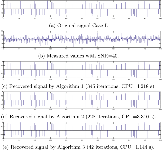

  

  Computational results for Example 4.5 Case IV

• (b) In Fig. 12, we plotted the mean squared error (MSE) value per iteration. It is evident that the errors obtained by Algorithm 3 decrease faster than for the other proposed algorithms.

  Figure 12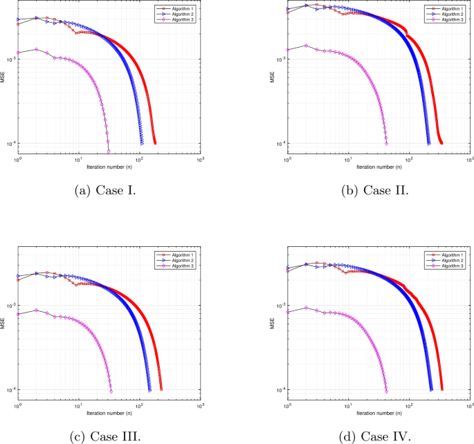

  

  Convergence behavior of MSE for Example 4.5

5 Conclusions

This work proposed three modified step size algorithms to solve the SEPs. These iterative algorithms were developed to approximate solutions for the SEPs with no prior knowledge. Strong convergence theorems are well established and proved under appropriate conditions. We gave some of the applications to solve the split feasibility problem and optimization problem. Numerical examples were presented to show the usefulness of our main results. Moreover, we showed the computational performance of the proposed algorithms by comparing them with the existing algorithms. The compared results show that the proposed algorithms outperform the state-of-the-art algorithms.

References

He, Z.: The split equilibrium problem and its convergence algorithms. J. Inequal. Appl. 2012(1), 162 (2012)
Ceng, L.C., Yao, J.C.: A hybrid iterative scheme for mixed equilibrium problems and fixed point problems. J. Comput. Appl. Math. 214(1), 186–201 (2008)
Combettes, P.L., Hirstoaga, S.A., et al.: Equilibrium programming in Hilbert spaces. J. Nonlinear Convex Anal. 6(1), 117–136 (2005)
Peng, J.W., Liou, Y.C., Yao, J.C.: An iterative algorithm combining viscosity method with parallel method for a generalized equilibrium problem and strict pseudocontractions. Fixed Point Theory Appl. 2009(1), 794178 (2009)
Tada, A., Takahashi, W.: Strong convergence theorem for an equilibrium problem and a nonexpansive mapping. J. Nonlinear Convex Anal., 609–617 (2007)
He, Z.H., Sun, J.T.: The problem of split convex feasibility and its alternating approximation algorithms. Acta Math. Sin. Engl. Ser. 31(12), 2353 (2015)
Kazmi, K., Rizvi, S.: Iterative approximation of a common solution of a split equilibrium problem, a variational inequality problem and a fixed point problem. J. Egypt. Math. Soc. 21(1), 44–51 (2013)
Suantai, S., Cholamjiak, P., Cho, Y.J., Cholamjiak, W.: On solving split equilibrium problems and fixed point problems of nonspreading multi-valued mappings in Hilbert spaces. Fixed Point Theory Appl. 2016(1), 1 (2016)
Onjai-Uea, N., Phuengrattana, W.: On solving split mixed equilibrium problems and fixed point problems of hybrid-type multivalued mappings in Hilbert spaces. J. Inequal. Appl. 2017(1), 1 (2017)
Deepho, J., Martínez-Moreno, J., Sitthithakerngkiet, K., Kumam, P.: Convergence analysis of hybrid projection with Cesàro mean method for the split equilibrium and general system of finite variational inequalities. J. Comput. Appl. Math. 318, 658–673 (2017)
Hieua, D.V.: Parallel extragradient-proximal methods for split equilibrium problems. Math. Model. Anal. 21(4), 478–501 (2016)
Moudafi, A.: Proximal point algorithm extended to equilibrium problems. J. Nat. Geom. 15(1–2), 91–100 (1999)
López, G., Martín Márquez, V., Wang, F., Xu, H.K.: Solving the split feasibility problem without prior knowledge of matrix norms. Inverse Probl. 28(8), 085004 (2012)
Yang, Q.: On variable-step relaxed projection algorithm for variational inequalities. J. Math. Anal. Appl. 302(1), 166–179 (2005)
Cianciaruso, F., Marino, G., Muglia, L., Yao, Y.: A hybrid projection algorithm for finding solutions of mixed equilibrium problem and variational inequality problem. Fixed Point Theory Appl. 2010(1), 383740 (2009)
Suzuki, T.: Strong convergence of Krasnoselskii and Mann’s type sequences for one-parameter nonexpansive semigroups without Bochner integrals. J. Math. Anal. Appl. 305(1), 227–239 (2005)
Opial, Z.: Weak convergence of successive approximations for nonexpansive mappings. Bull. Am. Math. Soc. 73, 531–537 (1967)
Xu, H.K.: Iterative algorithms for nonlinear operators. J. Lond. Math. Soc. 66(1), 240–256 (2002)
Maingé, P.E.: Strong convergence of projected subgradient methods for nonsmooth and nonstrictly convex minimization. Set-Valued Anal. 16(7–8), 899–912 (2008)
Censor, Y., Elfving, T.: A multiprojection algorithm using Bregman projections in a product space. Numer. Algorithms 8, 221–239 (1994)
Ansari, Q.H., Rehan, A.: Split feasibility and fixed point problems. In: Nonlinear Analysis, pp. 281–322. Springer, Berlin (2014)
Ansari, Q.H., Rehan, A.: Iterative methods for generalized split feasibility problems in Banach spaces. Carpath. J. Math. 33(1), 9–26 (2017)
Ceng, L.C., Ansari, Q.H., Yao, J.C.: An extragradient method for solving split feasibility and fixed point problems. Comput. Math. Appl. 64(4), 633–642 (2012)
Censor, Y., Bortfeld, T., Martin, B., Trofimov, A.: A unified approach for inversion problems in intensity-modulated radiation therapy. Phys. Med. Biol. 51(10), 2353 (2006)
Acknowledgements
The authors would like to thank the Department of Mathematics, Faculty of Applied Science, King Mongkut’s University of Technology North Bangkok.
Funding
This research project was supported by the Thailand Science Research and Innovation Fund, the University of Phayao (Grant No. FF65-RIM041); National Science, Research and Innovation Fund (NSRF), and King Mongkut’s University of Technology North Bangkok with Contract no. KMUTNB-FF-66-05.
Author information
Authors and Affiliations
Contributions
Conceptualization, KS, NK; Formal analysis, KS, NK; Investigation, KS, AJ; Software, SM, NK; Validation, SM, KS; Writing the original draft, KS, NK, AJ. All authors read and approved the final manuscript.
Corresponding author
Ethics declarations
Competing interests
The authors declare that they have no competing interests.
Rights and permissions
Open Access This article is licensed under a Creative Commons Attribution 4.0 International License, which permits use, sharing, adaptation, distribution and reproduction in any medium or format, as long as you give appropriate credit to the original author(s) and the source, provide a link to the Creative Commons licence, and indicate if changes were made. The images or other third party material in this article are included in the article’s Creative Commons licence, unless indicated otherwise in a credit line to the material. If material is not included in the article’s Creative Commons licence and your intended use is not permitted by statutory regulation or exceeds the permitted use, you will need to obtain permission directly from the copyright holder. To view a copy of this licence, visit http://creativecommons.org/licenses/by/4.0/.
About this article
Cite this article
Mekruksavanich, S., Kaewyong, N., Jitpattanakul, A. et al. Adapting step size algorithms for solving split equilibrium problems with applications to signal recovery. J Inequal Appl 2022, 125 (2022). https://doi.org/10.1186/s13660-022-02860-7
Received:
Accepted:
Published:
DOI: https://doi.org/10.1186/s13660-022-02860-7