Error-constant estimation under the maximum norm for linear Lagrange interpolation

Abstract

For the linear Lagrange interpolation over a triangular domain, we propose an efficient algorithm to rigorously evaluate the interpolation error constant under the maximum norm by using the finite-element method (FEM). In solving the optimization problem corresponding to the interpolation error constant, the maximum norm in the constraint condition is the most difficult part to process. To handle this difficulty, a novel method is proposed by combining the orthogonality of the space decomposition using the Fujino–Morley FEM space and the convex-hull property of the Bernstein representation of functions in the FEM space. Numerical results for the lower and upper bounds of the interpolation error constant for triangles of various types are presented to verify the efficiency of the proposed method.

1 Introduction

In this paper, we consider the error estimation for the linear Lagrange interpolation over triangle elements and provide explicit values for the error constant in the error estimation under the $L^{\infty}$-norm.

Before the detailed discussion of our results, let us introduce the existing literature on the Lagrange interpolation function in a general scope.

• (1D case) Given a 1-dimensional interval $I=(0,1)$, since $H^{1}(I)\subset C(\overline{I})$, we can define the Lagrange interpolation $\Pi ^{L} u$ such that $\Pi ^{L} u$ is a linear function satisfying $(u - \Pi ^{L} u)(0) =(u - \Pi ^{L} u)(1) =0$. Then, the following results are well known as optimal estimates if u is regular enough in the sense that the right-hand sides of the inequalities are well defined:

  $$\begin{aligned} & \bigl\lVert u-\Pi ^{L} u \bigr\rVert _{0,I} \le \frac{1}{\pi ^{2}} \lvert u \rvert _{2,I},\qquad \bigl\lvert u-\Pi ^{L} u \bigr\rvert _{1,I} \le \frac{1}{\pi} \lvert u \rvert _{2,I}, \\ & \bigl\lVert u-\Pi ^{L} u \bigr\rVert _{\infty,I} \le \frac{1}{8} \bigl\lVert u^{(2)} \bigr\rVert _{\infty,I}, \end{aligned}$$

  where $u^{(2)}$ denotes the second derivative of u, $\lVert \cdot \rVert _{0,I}$ and $\lVert \cdot \rVert _{\infty,I}$ denote the $L^{2}$- and $L^{\infty}$-norms, respectively, and $\lvert \cdot \rvert _{1,I}$ and $\lvert \cdot \rvert _{2,I}$ denote the $H^{1}$- and $H^{2}$-seminorms, respectively. The estimations presented above are optimal in the sense that there exist functions for which the equalities hold.

  • Let $u(x):= \sin (\pi x)$ on the interval $(0,1)$. Then, $\Pi ^{L} u(x) = 0$. In this case,

    $$\begin{aligned} \bigl\lVert u - \Pi ^{L} u \bigr\rVert _{0,I} = \frac{1}{\pi ^{2}} \lvert u \rvert _{2,I},\qquad \bigl\lvert u - \Pi ^{L} u \bigr\rvert _{1,I} = \frac{1}{\pi} \lvert u \rvert _{2,I} . \end{aligned}$$

  • Let $u(x):= x^{2}$ on the interval $(0,1)$. Then, $\Pi ^{L} u (x) = x$. In this case,

    $$\begin{aligned} \bigl\lVert u-\Pi ^{L}u \bigr\rVert _{\infty,I} = \frac{1}{8} \bigl\lVert u^{(2)} \bigr\rVert _{\infty,I}. \end{aligned}$$

• (2D case) Over a triangle K with vertices $p_{i}$ ($i=1,2,3$), the Lagrange interpolation function $\Pi ^{L} u$ is the linear function such that (see Fig. 1)

  $$\begin{aligned} \bigl(u-\Pi ^{L} u\bigr) (p_{i})=0,\quad \forall i=1,2,3. \end{aligned}$$

  Figure 1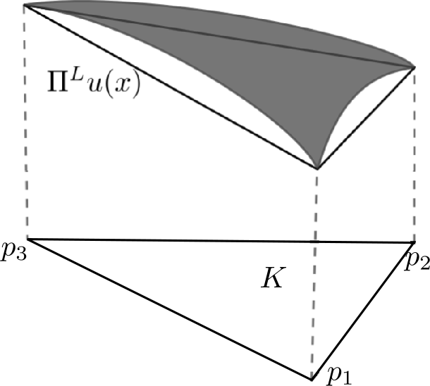

  

  A linear Lagrange interpolation function $\Pi ^{L} u$ defined on a triangle K

  In the case of $L^{2}$-norm and $H^{1}$-seminorm error estimation of $\Pi ^{L}$, one needs to estimate the interpolation error constants appearing in the following inequalities:

  $$\begin{aligned} \bigl\lVert u-\Pi ^{L} u \bigr\rVert _{0,K} \le C_{0}(K) \lvert u \rvert _{2,K},\qquad \bigl\lvert u-\Pi ^{L} u \bigr\rvert _{1,K} \le C_{1}(K) \lvert u \rvert _{2,K}. \end{aligned}$$

  Let h be the medium edge length of K, θ the maximum angle, and αh ($0<\alpha \le 1$) the smallest edge length. Kikuchi and Liu [1, 2] obtained a bound of $C_{0}$ and $C_{1}$ as follows:

  $$\begin{aligned} C_{0}(K) \le \frac{h}{\pi}\sqrt{1+ \lvert \cos \theta \rvert }, C_{1}(K) \le 0.493h \frac{1+\alpha ^{2}+\sqrt{1+2\alpha ^{2}\cos 2\theta + \alpha ^{4}}}{\sqrt{2 (1+\alpha ^{2}-\sqrt{1+2\alpha ^{2}\cos 2\theta +\alpha ^{4}} )}}. \end{aligned}$$

  Also, Kobayashi [3] showed that for a triangle K with edge lengths $A,B,C$ and area S, the following holds:

  $$\begin{aligned} \bigl\lvert u - \Pi ^{L} u \bigr\rvert _{1,K} \le C_{1}(K) \lvert u \rvert _{2,K}, \quad\forall u \in H^{2}(K), \end{aligned}$$

  where the constant $C_{1}(K)$ is defined by

  $$\begin{aligned} C_{1}(K):= \sqrt{\frac{A^{2}B^{2}C^{2}}{16S^{2}} - \frac{A^{2} + B^{2} + C^{2}}{30}- \frac{S^{2}}{5} \biggl( \frac{1}{A^{2}} + \frac{1}{B^{2}} + \frac{1}{C^{2}} \biggr)}. \end{aligned}$$

  The optimal estimation of constants $C_{0}(K)$ and $C_{1}(K)$ for a concrete K can be obtained by solving the corresponding eigenvalue problems with rigorous lower eigenvalue bounds; see the results of [4, 5].

  For $L^{\infty}$-norm error estimation under the $L^{\infty}$-norm of objective function, Waldron [6] provides the following sharp inequality:

  $$\begin{aligned} \bigl\lVert u - \Pi ^{L} u \bigr\rVert _{\infty,K} \le \frac{1}{2}\bigl(R^{2} - d^{2}\bigr) \bigl\lVert u^{(2)} \bigr\rVert _{\infty,K}, \end{aligned}$$

  (1)

  where R is the radius of the circumscribed circle of K, d is the distance of the center c of the circumscribed circle from K, and $\lVert u^{(2)} \rVert _{\infty,K}$ is defined by

  $${\parallel u^{(2)}\parallel }_{\mathrm{\infty },K}:=\underset{x\in K}{sup}\underset{\begin{array}{c}u,v\in {\mathbb{R}}^2\\ \parallel u\parallel =\parallel v\parallel =1\end{array}}{sup}|D_u{D}_{v}u(x)|=\underset{x\in K}{sup}\underset{\begin{array}{c}\xi \in {\mathbb{R}}^2\\ \parallel \xi \parallel =1\end{array}}{sup}|D_{\xi }^{2}u(x)|.$$

  In particular, if $c \in K$,

  $$\begin{aligned} \bigl\lVert u - \Pi ^{L} u \bigr\rVert _{\infty, K} \le \frac{1}{2}R^{2} \bigl\lVert u^{(2)} \bigr\rVert _{\infty,K}. \end{aligned}$$

  A detailed discussion on the $L^{\infty}$-norm of interpolation error for a quadratic polynomial f is considered by D’Azevedo and Simpson [7]. In [8], Shewchuk gives a survey of the interpolation error estimation with $L^{\infty}$-norm for both $f-\Pi ^{L} f$ and $\nabla (f-\Pi ^{L} f)$, along with the discussion on the relation between the interpolation error and the finite-element approximation of error functions. Also, the discussion on the affection of the aspect ratio of a triangle element to the interpolation error can be found in Cao [9].

In this research, we consider the $L^{\infty}$-norm estimation for the Lagrange interpolation over triangle element K by using the $H^{2}$-seminorm of the objective function, that is,

$$\begin{aligned} \bigl\lVert u-\Pi ^{L} u \bigr\rVert _{\infty,K} \le C^{L}(K) \lvert u \rvert _{2,K}, \quad\forall u \in H^{2}(K). \end{aligned}$$

(2)

Here, $C^{L}(K)$ is the interpolation error constant to be evaluated explicitly. Note that since $W^{2,\infty}(K) \subseteq H^{2}(K)$, the inequality (2) is more general than Waldron’s result (1). In this paper, it is aimed to give sharp estimation for the constant $C^{L}(K)$. For example, for the unit isosceles right triangle element, the following estimation holds for the optimal constant $C^{L}(K)$ in (2):

$$\begin{aligned} 0.40432 \le C^{L}(K) \le 0.41596. \end{aligned}$$

Estimation of $C^{L}(K)$ for triangles of general shapes is provided in Theorem 2.3, while sharp bounds for concrete triangles are discussed in Sect. 3. Such a kind of estimation is helpful to provide explicit maximum norm error estimation for the FEM solution to boundary value problems by further applying the point-wise error estimation (see, e.g., [10]), which will be considered in our succeeding work; see also classical qualitative error analysis under the maximum norm in Sects. 19–22 of [11];

The contribution of our paper is summarized as follows.

• (1) For triangle element K of general shapes, a formula to give an upper bound of $C^{L}(K)$ is obtained by theoretical analysis. The bound is raw but works well for triangle elements of arbitrary shapes. In particular, our analysis tells us that the value of $C^{L}(K)$ can be very large and tends to ∞ if the triangle element tends to degenerate to a 1D segment; see detail in Sect. 2.2.

• (2) For a specific triangle element K, the optimal estimation of $C^{L}(K)$ is obtained by solving the corresponding optimization problem over $H^{2}(K)$ under the constraint condition involving $L^{\infty}$-norm. The processing of the constraint condition with $L^{\infty}$-norm is not an easy task. We develop a novel algorithm to provide efficient and sharp estimation for the solution of the optimization problem. With a light computation, one can obtain the estimation of $C^{L}(K)$ with relative error less than 1%.

The rest of our paper is structured as follows. At the end of this section, we introduce the preliminary concepts and notations to be used throughout the paper. In Sect. 2, the estimation of the upper bound for $C^{L}(K)$ is considered using a theoretical approach. The raw upper bound of the interpolation error constant is calculated for a right isosceles triangle. Also, we investigate the asymptotic behavior of the constant as the triangle tends to degenerate. In Sect. 3, using a finite-element method (FEM), an algorithm for the optimal estimation of the constant is proposed. Lower bounds for the constant are calculated to confirm the efficiency of the proposed algorithm. The numerical results are summarized and the conclusion is presented in Sect. 4.

Notation

Let us introduce the notation for the function spaces used in this paper. In most cases, the domain Ω of functions is selected as a triangle element K. The standard notation is used for Sobolev function spaces $W^{k,p}(\Omega )$. The associated norms and seminorms are denoted by $\lVert \cdot \rVert _{k,p,\Omega}$ and $\lvert \cdot \rvert _{k,p,\Omega}$, respectively (see, e.g., Chap. 1 of [12] and Chap. 1 of [13]). In particular, for special k and p, we use abbreviated notations as $H^{k}(\Omega )=W^{k,2}(\Omega )$, $\lvert \cdot \rvert _{k,\Omega} = \lvert \cdot \rvert _{k,2,\Omega}$, and $L^{p}(\Omega )=W^{0,p}(\Omega )$. The set of polynomials over K of up to degree k is denoted by $P_{k}(K)$. The second-order derivative is given by $D^{2} u:= ( u_{xx}, u_{xy}, u_{yx}, u_{yy})$ for $u \in H^{2}(K)$.

Given a triangle K, denote each vertex by $p_{i}$ ($i=1,2,3$) and the largest edge length by $h_{K}$; see Fig. 2. We follow the notation introduced by Liu and Kikuchi [2] to configure a general triangle with geometric parameters. Let $h, \alpha$, and θ be positive constants such that

$$\begin{aligned} h>0, 0 < \alpha \le 1, \quad\biggl(\frac{\pi}{3} \le \biggr) \cos ^{-1} \biggl(\frac{\alpha}{2} \biggr) \le \theta < \pi. \end{aligned}$$

Define a triangle $K_{\alpha,\theta,h}$ with three vertices $p_{1}(0,0)$, $p_{2}(h,0)$, and $p_{3}(\alpha h \cos \theta, \alpha h \sin \theta )$. Note that $h \le h_{K}$. In the case of $h=1$, the notation $K_{\alpha,\theta,1}$ is abbreviated as $K_{\alpha,\theta}$.

Figure 2

Configuration of triangle $K_{\alpha,\theta,h}$

With the above configuration of the triangle $K_{\alpha,\theta,h}$, the optimal constant $C^{L}(K)$ in (2) can be defined as follows:

$$\begin{aligned} C^{L}(\alpha,\theta,h):= \sup_{u\in H^{2}(K_{\alpha,\theta,h})} \frac{ \lVert u-\Pi ^{L} u \rVert _{\infty,K_{\alpha,\theta,h}} }{ \lvert u \rvert _{2,K_{\alpha,\theta,h}}} . \end{aligned}$$

(3)

By scaling of the triangle element, it is easy to confirm that $C^{L}(\alpha,\theta,h)=h C^{L}(\alpha,\theta,1)$.

In the rest of the paper, we show how to obtain explicit bounds for the error constant $C^{L}(\alpha,\theta,h)$.

2 Raw upper bound of the constant

In this section, a raw upper bound of the constant is obtained through theoretical analysis. Such a bound applies to triangles of arbitrary shapes.

First, let us quote a lemma about the trace theorem, which gives an estimation for the integral over edge of a triangle element. For the reader’s convenience, we show the proof in a concise way; refer to, e.g., [14–16] for more detailed discussion.

Lemma 2.1

(Trace theorem)

Let e be one of the edges of triangle K; see Fig. 3. Given $w\in H^{1}({K})$, we have the following estimation:

$$\begin{aligned} \lVert w \rVert ^{2}_{0,e} \le \frac{ \lvert e \rvert }{ \lvert K \rvert } \bigl\{ \lVert w \rVert _{0,K}^{2} + h_{K} \lVert w \rVert _{0,K} \lvert w \rvert _{1,K} \bigr\} . \end{aligned}$$

Figure 3

A triangle K with base e and height $H_{K}$

Proof

For any $w \in H^{1}(K)$, the Green theorem leads to

$$\begin{aligned} \int _{K} \bigl((x,y)- p_{3} \bigr) \cdot \nabla \bigl(w^{2}\bigr) \,\mathrm{d}K = \int _{ \partial K} \bigl((x,y)- p_{3} \bigr)\cdot { \overrightarrow{n}} w^{2} \,\mathrm{d}s - \int _{K} 2 w^{2} \,\mathrm{d} K. \end{aligned}$$

Here, $\overrightarrow{n}$ is the unit outer normal direction on the boundary of K. For the term $((x,y)- p_{3} )\cdot {\overrightarrow{n}}$, we have

$$\begin{aligned} \bigl((x,y)- p_{3} \bigr)\cdot {\overrightarrow{n}} = \textstyle\begin{cases} 0 & \mbox{on } p_{1}p_{3}, p_{2}p_{3}, \\ H_{K} & \mbox{on } e. \end{cases}\displaystyle \end{aligned}$$

Here, $H_{K}$ is the height of the triangle with base as e. Thus,

$$\begin{aligned} H_{K} \int _{e} w^{2} \,\mathrm{d} s & = \int _{K} 2 w^{2} \,\mathrm{d} K + \int _{K} \bigl((x,y)- p_{3} \bigr) \cdot \nabla \bigl(w^{2}\bigr) \,\mathrm{d} K \\ & \le \int _{K} 2 w^{2} \,\mathrm{d} K + 2h_{K} \int _{K} w \lvert \nabla w \rvert \,\mathrm{d} K \\ & \le 2 \lVert w \rVert _{0,K}^{2} + 2h_{K} \lVert w \rVert _{0,K} \lVert \nabla w \rVert _{0,K}. \end{aligned}$$

We can now draw the conclusion by sorting the above inequality. □

Using the trace theorem, the following result provides a pointwise estimation of the interpolation error.

Lemma 2.2

Given $u\in H^{2}(K)$, for any point $\mathbf{x}_{0} \in K$, we have

$$\begin{aligned} \bigl\lvert \bigl(u-\Pi ^{L} u\bigr) (\mathbf{x}_{0}) \bigr\rvert \le \frac {\sqrt{2 \lvert p_{1}\mathbf{x}_{0} \rvert }}{\sqrt{H_{\widetilde{K}}}} \bigl(h_{K} \bigl\lvert u-\Pi ^{L} u \bigr\rvert _{1,K} \lvert u \rvert _{2,K} + \bigl\lvert u-\Pi ^{L} u \bigr\rvert _{1,K}^{2} \bigr)^{\frac{1}{2}}, \end{aligned}$$

where $h_{K}$ is the longest edge length of K, and $H_{\widetilde{K}}$ is the height of the subtriangle $\widetilde{K} = p_{1}\mathbf{x}_{0} p_{3}$ with respect to the base $\tilde{e} = p_{1}\mathbf{x}_{0}$ (see Fig. 4).

Figure 4

A subtriangle K̃ in a triangle K

Proof

Let $g = u - \Pi ^{L} u$ and t be the direction along edge $p_{1} \mathbf{x}_{0}$. In Lemma 2.1, by taking $w:=\frac{\partial g}{\partial t}$, we have

$$\begin{aligned} \biggl\lVert \frac{\partial g}{\partial t} \biggr\rVert ^{2}_{0, \tilde{e}} \le \frac{ \lvert \tilde{e} \rvert }{\lvert \widetilde{K}\rvert} \bigl( \lVert w \rVert ^{2}_{0,\widetilde{K}} + h_{ \widetilde{K}} \lVert w \rVert _{0,\widetilde{K}} \lvert w \rvert _{1,\widetilde{K}} \bigr) \le \frac{ \lvert \tilde{e} \rvert }{\lvert \widetilde{K}\rvert} \bigl( \lvert g \rvert ^{2}_{1,\widetilde{K}} + h_{ \widetilde{K}} \lvert g \rvert _{1,\widetilde{K}} \lvert g \rvert _{2,\widetilde{K}} \bigr). \end{aligned}$$

Taking the Taylor expansion of g on the segment ẽ and noting that $g(p_{1}) = 0$,

$$\begin{aligned} \bigl\lvert g(\mathbf{x}_{0}) \bigr\rvert & = \biggl\lvert \int _{p_{1}\mathbf{x}_{0}} \frac {\partial g}{\partial t}\,\mathrm{d}t + g(p_{1}) \biggr\rvert \le \sqrt{ \lvert p_{1}\mathbf{x}_{0} \rvert } \cdot \biggl\lVert \frac{\partial g}{\partial t} \biggr\rVert _{0,\tilde{e}} \\ & \leq \frac { \lvert p_{1}\mathbf{x}_{0} \rvert }{\sqrt{ \vert \widetilde{K} \vert }} \bigl(h_{K} \lvert g \rvert _{1,\widetilde{K}} \lvert g \rvert _{2,\widetilde{K}} + \lvert g \rvert _{1,\widetilde{K}}^{2} \bigr)^{\frac{1}{2}} \\ & \le \frac{\sqrt{2 \lvert p_{1}\mathbf{x}_{0} \rvert }}{\sqrt{H_{\widetilde{K}}}} \bigl(h_{K} \lvert g \rvert _{1,K} \lvert g \rvert _{2,K} + \lvert g \rvert _{1,K}^{2} \bigr)^{ \frac{1}{2}}. \end{aligned}$$

The conclusion follows. □

Liu and Kikuchi [2] considered the estimation of the constant $C_{1}(\alpha,\theta )$ for different types of triangles $K = K_{\alpha,\theta}$ such that

$$\begin{aligned} \bigl\lvert u - \Pi ^{L} u \bigr\rvert _{1,K}\le C_{1}(\alpha, \theta ) h \lvert u \rvert _{2,K},\quad \forall u \in H^{2}(K), \end{aligned}$$

where h is the medium length of K. The constant $C_{1}(\alpha,\theta )$ is used to give a bound for $C^{L}(K)$, as shown in the lemma below.

Lemma 2.3

Given $u \in H^{2}(K)$, for any point $\mathbf{x}_{0} \in K$, we have

$$\begin{aligned} \bigl\lvert \bigl(u -\Pi ^{L} u\bigr) ( \mathbf{x}_{0}) \bigr\rvert \le \frac{\sqrt{2 \lvert p_{1} \mathbf{x}_{0} \rvert }}{\sqrt{H_{\widetilde{K}}}} \bigl(C_{1}(\alpha,\theta )hh_{K} + C^{2}_{1}( \alpha,\theta )h^{2} \bigr)^{\frac{1}{2}} \lvert u \rvert _{2,K}. \end{aligned}$$

(4)

2.1 The case for a right isosceles triangle

Using Lemma 2.3, we obtain the upper bound of the constant for right isosceles triangles: For the right isosceles triangle $K=K_{1,\frac{\pi}{2},h}$,

$$\begin{aligned} \bigl\lVert u - \Pi ^{L} u \bigr\rVert _{\infty,K} \le 1.3712h \lvert u \rvert _{2,K}. \end{aligned}$$

(5)

Suppose a point $\mathbf{x}_{0}$ subdivides K into $K_{1}, K_{2}, K_{3}$; see Fig. 5. Let us consider the estimation of the term $\lvert p_{1}\mathbf{x}_{0} \rvert /H_{K_{2}}$, which is required in Lemma 2.3. Let $p_{1}p_{4}$ be the height of K with base as $p_{2} p_{3}$. Due to the symmetry of K, it is enough to only consider the case that $\mathbf{x}_{0} \in K$ is below the line $p_{1}p_{4}$. Let p be the intersection of the extended line of $p_{1}\mathbf{x}_{0}$ and edge $p_{2}p_{3}$. Note that $\lvert p_{1}\mathbf{x}_{0} \rvert \le \lvert p_{1}p \rvert$. For $p:=(\overline{x},\overline{y})$ on $p_{2}p_{4}$, $\lvert p_{1}p \rvert = \sqrt{\overline{x}^{2}+ \overline{y}^{2}}$. The height of $K_{2}$ with base $p_{1}\mathbf{x}_{0}$ is given by

$$\begin{aligned} H_{K_{2}} = \frac{h\overline{x}}{\sqrt{\overline{x}^{2}+\overline{y}^{2}}}. \end{aligned}$$

Figure 5

A right isosceles triangle $K_{1,\frac{\pi}{2},h}$

Then, since $\overline{y} = h-\overline{x}$,

$$\begin{aligned} \frac{ \lvert p_{1}p \rvert }{H_{K_{2}}} = \frac{2\overline{x}^{2}-2h\overline{x}+h^{2}}{h\overline{x}}. \end{aligned}$$

The above quantity takes its maximum value at $p = (\frac{h}{2},\frac{h}{2} )$ and $p = (h,0)$, and its maximum value is 1. Thus, for any p on $p_{2}p_{4}$, $\lvert p_{1}p \rvert /H_{K_{2}} \le 1$. From [2], $C_{1} (1,\frac{\pi}{2} ) \le 0.49293$. Since $h_{K} = \sqrt{2}h$, by inequality (4),

$$\begin{aligned} \bigl\lvert \bigl(u -\Pi ^{L} u\bigr) (\mathbf{x}_{0}) \bigr\rvert \le \sqrt{2} \bigl[(0.49293)\sqrt{2} + 0.49293^{2} \bigr]^{\frac{1}{2}} h \lvert u \rvert _{2,K} \le 1.3712h \lvert u \rvert _{2,K}. \end{aligned}$$

Hence, we obtain the error estimate for a right isosceles triangle as in (5).

2.2 Dependence of the constant on the shape of K

In this subsection, we consider the variation of the interpolation constant when a reference triangle, i.e., the right isosceles triangle, is transformed to a general triangle.

Theorem 2.1

For a general element $K_{\alpha,\theta}$, the following estimation for constant $C^{L}(\alpha, \theta )$ holds:

$$\begin{aligned} C^{L}(\alpha, \theta ) \le \frac{v_{+}(\alpha, \theta )}{2\sqrt{\alpha \sin \theta}} C^{L} \biggl(1,\frac{\pi}{2} \biggr), \end{aligned}$$

(6)

where $v_{+}(\alpha, \theta ) = 1 + \alpha ^{2} + \sqrt{1+2\alpha ^{2} \cos 2\theta + \alpha ^{4}}$.

Proof

Let us consider the affine transformation between $x = (x_{1},x_{2}) \in K_{\alpha,\theta}$ and $\xi = (\xi _{1},\xi _{2}) \in K_{1,\frac{\pi}{2}}$:

$$\begin{aligned} \xi _{1} = x_{1} - \frac{x_{2}}{\tan \theta},\qquad \xi _{2} = \frac{x_{2}}{\alpha \sin \theta} \quad\mbox{or}\quad x_{1} = \xi _{1} + \alpha \xi _{2} \cos \theta,\qquad x_{2} = \alpha \xi _{2} \sin \theta. \end{aligned}$$

Given $\tilde{v}(\xi )$ over $K_{1,\frac{\pi}{2}}$, define $v(x)$ over $K_{\alpha,\theta}$ by $v(x_{1},x_{2}) = \tilde{v}(\xi _{1}, \xi _{2})$. Thus,

$$\begin{aligned} \lVert v \rVert _{\infty, K_{\alpha,\theta}} = \lVert \tilde{v} \rVert _{\infty, K_{1,\frac{\pi}{2}}}. \end{aligned}$$

The estimation for the variation of $H^{2}$-seminorm in Theorem 1 of [2] tells us that

$$\begin{aligned} \lvert v \rvert _{2, K_{\alpha,\theta}} \ge \frac{2 \sqrt{\alpha \sin \theta}}{v_{+}(\alpha,\theta )} \lvert \tilde{v} \rvert _{2,K_{1,\frac{\pi}{2}}}. \end{aligned}$$

Thus, we draw the conclusion from the definition of constant $C^{L}(\alpha,\theta )$ in (3). □

Lemma 2.4

For shape-regular triangles, $C^{L}(\alpha, \theta )$ is bounded. Here, by “shape-regular triangles” it means that for a certain positive quantity δ, the minimal inner angle of each triangle, denoted by $\theta _{\mathrm{min}}$, the inequality $\theta _{\mathrm{min}} \ge \delta$ holds.

Proof

It is easy to see that for all triangles with $\theta _{\mathrm{min}} \ge \delta$, the term $v_{+}(\alpha,\theta )/\sqrt{\alpha \sin \theta}$ in (6) is uniformly bounded. As $C^{L}(1,\pi /2)$ has a finite value, we draw the conclusion from the estimation (6). □

Remark 2.1

By using the raw bound of $C^{L} (1,\frac{\pi}{2} ) \le 1.3712 h$ in (5), an explicit but raw bound of $C^{L}(\alpha,\theta )$ is available. Later, with a sharp and rigorous estimation of $C^{L} (1,\frac{\pi}{2} )$ based on a numerical approach, the bound can be improved as

$$\begin{aligned} C^{L}(\alpha, \theta,h) \le 0.41596 h \frac{v_{+}(\alpha, \theta )}{2\sqrt{\alpha \sin \theta}}. \end{aligned}$$

(7)

Remark 2.2

Here are two remarks on the asymptotic behavior of the constant when the triangle degenerates to a segment.

• 1. Suppose the maximum inner angle θ of $K_{\alpha,\theta}$ is close to π; see Fig. 6. Let $u(x,y):= x^{2} + y^{2}$. Then, $\Pi ^{L} u (x,y) = x + ((\alpha - \cos \theta )/\sin \theta ) y$ and

  $$\begin{aligned} \bigl\lVert u - \Pi ^{L} u \bigr\rVert _{\infty,K_{\alpha,\theta}} = \bigl(2\alpha \cos \theta - \alpha ^{2} - 1\bigr)/4, \qquad\lvert u \rvert _{2,K_{\alpha,\theta}} = 2 \sqrt{\alpha \sin \theta}. \end{aligned}$$

  Thus, we have a lower bound of $C^{L}(\alpha,\theta )$ as follows,

  $$\begin{aligned} C^{L}(\alpha,\theta ) \ge \frac{2\alpha \cos \theta - \alpha ^{2} -1}{8\sqrt{\alpha \sin \theta}} . \end{aligned}$$

  In this case, $C^{L}(\alpha,\theta )$ diverges to ∞ as θ tends to π.

  Figure 6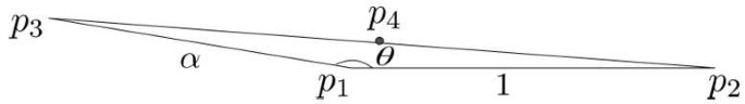

  

  A triangle $K_{\alpha,\theta}$ with angle θ close to π

• 2. For triangle $K_{\alpha, \frac{\pi}{2}}$ shown in Fig. 7, let $u(x,y):= \lvert (x,y)- p_{4} \rvert ^{2}$, where $p_{4}$ is the midpoint of the edge $p_{2}p_{3}$. Then, $\Pi ^{L} u = (\alpha ^{2} + 1)/4$ and

  $$\begin{aligned} \bigl\lVert u - \Pi ^{L} u \bigr\rVert _{\infty,K_{\alpha, \frac{\pi}{2}}} = \bigl(\alpha ^{2} +1\bigr)/4, \qquad\lvert u \rvert _{2,K_{\alpha, \frac{\pi}{2}}} = 2\sqrt{\alpha}. \end{aligned}$$

  Thus,

  $$\begin{aligned} \frac{ \lVert u - \Pi ^{L} u \rVert _{\infty,K_{\alpha, \frac{\pi}{2}}}}{ \lvert u \rvert _{2,K_{\alpha, \frac{\pi}{2}}}} = \frac{\alpha ^{2}+1}{8\sqrt{\alpha}} \biggl(\le C^{L} \biggl( \alpha,\frac{\pi}{2} \biggr) \biggr). \end{aligned}$$

  When $\alpha \to 0$, although the maximum inner angle is invariant, the interpolation error constant $C^{L} (\alpha,\frac{\pi}{2} )$ tends to ∞.

  Figure 7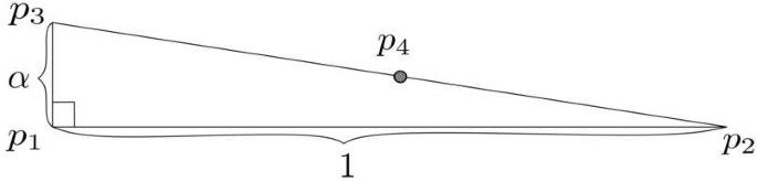

  

  A right triangle $K_{\alpha, \frac{\pi}{2}}$ with one leg length close to 0

3 Optimal estimation of the constant

In the previous section, we obtained explicit bounds for the interpolation constant for triangles of general shape. Basically, such bounds from theoretical analysis only provide a raw bound for the objective constant. In this section, we propose a numerical algorithm to obtain the optimal estimation of the constant $C^{L}(K)$ for specific triangles.

Let us define the space $V^{L}(K):= \{u \in H^{2}(K) \mid u(p_{i}) = 0 \ (i = 1,2,3) \}$. Let $\mathcal{T}^{h}$ be a triangulation of the domain K and define the space

$$\begin{aligned} V^{{F M}}_{h}(K):={}& \biggl\{ v \mid v \vert _{K_{h}} \in P_{2}(K_{h}), \forall {K_{h}} \in \mathcal{T}^{h}; v(p_{i}) = 0\ (i = 1,2,3); v \mbox{ is continuous} \\ &\mbox{at the nodes; } { \int _{e} \biggl(\frac{\partial v}{\partial \overrightarrow{n}} \bigg|_{K_{h}} - \frac{\partial v}{\partial \overrightarrow{n}} \bigg|_{K_{h}'} \biggr) \,\mathrm{d}s = 0 \mbox{ for each } e = K_{h} \cap K_{h'} } \biggr\} . \end{aligned}$$

For $u_{h}, v_{h} \in V^{{F M}}_{h}(K)$, define the discretized $H^{2}$-inner product and seminorm by

$$\begin{aligned} \langle u_{h}, v_{h} \rangle _{h}:= \sum _{{K_{h}} \in \mathcal{T}^{h}} \int _{{K_{h}}} D^{2}{u_{h}|_{K_{h}}} \cdot D^{2} {v_{h}|_{K_{h}}} \,\mathrm{d} {K_{h}},\quad \lvert u_{h} \rvert _{2,K}:= \sqrt{ \langle u_{h}, u_{h} \rangle _{h}} . \end{aligned}$$

Let us define the two quantities over the triangle K:

$$\begin{aligned} \lambda (K):= \inf_{u \in V^{L}(K)} \frac{ \lvert u \rvert _{2,K}^{2}}{ \lVert u \rVert _{\infty,K}^{2}},\qquad \lambda _{h}(K):= \min_{u_{h} \in V_{h}^{{F M}}(K)} \frac{ \lvert u_{h} \rvert _{2,K}^{2}}{ \lVert u_{h} \rVert _{\infty,K}^{2}}. \end{aligned}$$

(8)

Note that $C^{L}(K) = \sqrt{\lambda (K)}^{-1}$ holds. In Theorem 3.1, we describe the algorithm to bound λ by using $\lambda _{h}$.

Given $u \in H^{2}(K)$, the Fujino–Morley interpolation $\Pi ^{{F M}}_{h} u$ is a function satisfying

$$\begin{aligned} \Pi ^{{F M}}_{h} u \in V^{{F M}}_{h}(K);\qquad \Pi ^{{F M}}_{h} u |_{{K_{h}}} \in P_{2}(K_{h}),\quad \forall {K_{h}} \in \mathcal{T}^{h}, \end{aligned}$$

and at the vertices $p_{i}$ and edges $e_{i}$ of K,

$$\begin{aligned} \bigl(u - \Pi ^{{F M}}_{h} u\bigr) (p_{i}) = 0,\qquad \int _{e_{i}} \frac{\partial}{\partial n}\bigl(u - \Pi ^{{F M}}_{h} u\bigr) \,\mathrm{d}s = 0\quad (i = 1,2,3). \end{aligned}$$

The Fujino–Morley interpolation has the property that (see, e.g., [4, 5])

$$\begin{aligned} \bigl\langle u - \Pi ^{{F M}}_{h} u, v_{h} \bigr\rangle _{h} = 0, \quad\forall v_{h} \in V^{{F M}}_{h}(K). \end{aligned}$$

(9)

Let $V(h):= \{u + u_{h} \mid u \in V^{L}(K), u_{h} \in V^{ {F M}}_{h}(K) \}$. Thus, it is easy to see that the Fujino–Morley interpolation is just the projection $P_{h}: V(h)\to V^{{F M}}_{h}(K)$ with respect to the inner product $\langle \cdot, \cdot \rangle _{h}$.

Below, let us introduce the theorem that provides an explicit lower bound of λ. Such a result is inspired by the idea of [17] for the lower bounds of eigenvalue problems.

Let $C_{h}^{{F M}}$ be a quantity that makes the following inequality hold.

$$\begin{aligned} \bigl\lVert u - \Pi ^{{\scriptsize F M}}_{h} u \bigr\rVert _{ \infty,K} \le C^{{F M}}_{h} \bigl\lvert u - \Pi ^{{\scriptsize F M}}_{h} u \bigr\rvert _{2,K},\quad \forall u \in V^{L}(K). \end{aligned}$$

(10)

The existence of $C_{h}^{{F M}}$ is confirmed by the argument in Sect. 3.1.

Theorem 3.1

With the quantity $C_{h}^{{F M}}$, we have a lower bound of $\lambda (K)$ as follows:

$$\begin{aligned} \lambda (K) \ge \frac{\lambda _{h}}{1+(C_{h}^{{F M}})^{2}\lambda _{h}} . \end{aligned}$$

(11)

Proof

For any $u \in V^{L}(K)$, noting that $\lvert \Pi ^{{\scriptsize F M}}_{h} u \rvert _{2,K} \ge \sqrt{\lambda _{h}} \lVert \Pi ^{{\scriptsize F M}}_{h} u \rVert _{\infty,K}$ and applying the inequality (10), we have

$$\begin{aligned} \lVert u \rVert _{\infty,K}& = \bigl\lVert \Pi _{h}^{{ \scriptsize F M}}u + u-\Pi _{h}^{{\scriptsize F M}}u \bigr\rVert _{ \infty,K} \\ & \le \bigl\lVert \Pi _{h}^{{\scriptsize F M}}u \bigr\rVert _{ \infty,K} + \bigl\lVert u-\Pi _{h}^{{\scriptsize F M}}u \bigr\rVert _{\infty,K} \\ & \le \frac{ \lvert \Pi _{h}^{{\scriptsize F M}}u \rvert _{2,K}}{\sqrt{\lambda _{h}}} + C_{h}^{{F M}} \bigl\lvert u-\Pi _{h}^{{\scriptsize F M}}u \bigr\rvert _{2,K} \\ & \le \sqrt{\frac{1}{\lambda _{h}} + \bigl(C_{h}^{{F M}} \bigr)^{2}} \sqrt{ \bigl\lvert \Pi _{h}^{{\scriptsize F M}}u \bigr\rvert ^{2}_{2,K} + \bigl\lvert u-\Pi _{h}^{{\scriptsize F M}}u \bigr\rvert ^{2}_{2,K}} . \end{aligned}$$

From the orthogonality in (9), we have

$$\begin{aligned} \bigl\lvert \Pi _{h}^{{\scriptsize F M}}u \bigr\rvert ^{2}_{2,K} + \bigl\lvert u-\Pi _{h}^{{\scriptsize F M}}u \bigr\rvert ^{2}_{2,K} = \lvert u \rvert _{2,K}^{2}. \end{aligned}$$

Thus,

$$\begin{aligned} \lVert u \rVert _{\infty,K} \le \sqrt{ \frac{1+(C_{h}^{{F M}})^{2}\lambda _{h}}{\lambda _{h}}} \lvert u \rvert _{2,K}, \quad \forall u \in V^{L}(K). \end{aligned}$$

From the definition of λ in (8), we draw the conclusion. □

To apply Theorem 3.1 for bounding λ, an explicit value of $C_{h}^{{F M}}$ is needed. Below, let us describe the way to obtain this explicit value by utilizing the raw bound of $C^{L}(\alpha,\theta )$.

3.1 Explicit estimation of $C^{{F M}}_{h}$

To have an explicit value of $C^{{F M}}_{h}$, we first define the quantity $C^{{F M}}_{\mathrm{res}}({K_{h}})$ for each element ${K_{h}}$ in the triangulation $\mathcal{T}^{h}$:

$$\begin{aligned} C^{{F M}}_{\mathrm{res}}({K_{h}}):= \sup _{u \in H^{2}( {K_{h}})} \frac{ \lVert u-\Pi _{h}^{{\scriptsize F M}}u \rVert _{\infty, {K_{h}}}}{ \lvert u-\Pi _{h}^{{\scriptsize F M}}u \rvert _{2,{K_{h}}}} = \sup_{w \in W_{1}} \frac{ \lVert w \rVert _{\infty, {K_{h}}}}{ \lvert w \rvert _{2,{K_{h}}}}. \end{aligned}$$

Here, $W_{1}:= \{w \in H^{2}({K_{h}}) \mid w(p_{i}) = 0, \int _{e_{i}} \frac{\partial w}{\partial n }\,\mathrm{d}s = 0 \ (i = 1,2,3) \}$. Noting that $W_{1} \subseteq W_{2}$ for $W_{2}:= \{ w \in H^{2}({K_{h}}) \mid w(p_{i}) = 0 \ (i=1,2,3) \}$, from the definition of $C^{L}$ in (3), we have

$$\begin{aligned} C^{{F M}}_{\mathrm{res}}({K_{h}}) \le \sup _{w \in W_{2}} \frac{ \lVert w \rVert _{\infty, {K_{h}}}}{ \lvert w \rvert _{2,{K_{h}}}} = C^{L}( {K_{h}}). \end{aligned}$$

Then, the following $C^{{F M}}_{h}$ with an upper bound makes certain (10) holds:

$$\begin{aligned} C^{{F M}}_{h}:= \max_{{K_{h}} \in \mathcal{T}^{h}} C^{ {F M}}_{\mathrm{res}}({K_{h}}) \Bigl( \le \max _{{K_{h}} \in \mathcal{T}^{h}} C^{L}({K_{h}}) \Bigr). \end{aligned}$$

(12)

Remark 3.1

Let $\mathcal{T}^{h}$ be a uniform triangulation of a right isosceles triangle; see a sample mesh in Fig. 8. We choose an explicit upper bound of $C^{{F M}}_{h}$ as $C^{{F M}}_{h} \le 1.3712h$, since for each ${K_{h}} \in \mathcal{T}^{h}$, $C^{{F M}}_{\mathrm{res}} \le C^{L}({K_{h}}) \le 1.3712h$, where h is the leg length of each right triangle element.

Figure 8

A uniform triangulation of a right isosceles triangle

3.2 Estimation of $\lambda _{h}$ by solving the finite-dimensional optimization problem

In this subsection, we present a method to estimate $\lambda _{h}$, which is required in Theorem 3.1 for bounding λ. Let $M:= \operatorname{Dim}(V^{{F M}}_{h})$. The estimation of $\lambda _{h}$ is equivalent to finding the solution to the optimization problem

$$\begin{aligned} \lambda _{h} =\operatorname{min} \mathbf{x}^{T} \mathbf{A} \mathbf{x}, \quad\mbox{subject to}\quad \Biggl\lVert \sum _{i=1}^{M} \mathbf{x}_{i} \phi _{i} \Biggr\rVert _{\infty,K} \ge 1 , \end{aligned}$$

(13)

where the components $a_{ij}$ of A are given by $a_{ij} = \langle \phi _{i}, \phi _{j} \rangle _{h}$, $\{\phi _{i} \}_{i=1,\ldots,M}$ are the basis functions for the Fujino–Morley space $V^{{F M}}_{h}$, and $\mathbf{x}\in {\mathbb{R}}^M$ denotes the Fujino–Morley coefficient vector of $u_{h} \in V^{{F M}}_{h}$.

To solve the optimization problem (13) is not an easy task since the $L^{\infty}$-norm of the function appears in the constraint. Here, we introduce the technique to apply Bernstein polynomials and their convex-hull property to solve the problem. Strictly speaking, a new optimization problem (14) utilizing the Bernstein polynomials will be formulated to provide a lower bound for the solution of (13).

As preparation, let us introduce the definition of Bernstein polynomials along with the convex-hull property; refer to, e.g., [18, 19] for detailed discussion.

Convex-hull property of Bernstein polynomials

Given a triangle K, let $(u,v,w)$ be the barycentric coordinates for a point x in K. A Bernstein polynomial p of degree n over a triangle K is defined by

$$\begin{aligned} {p}:= \sum_{i+j+k = n} d_{i,j,k} J^{(n)}_{i,j,k},\qquad J^{(n)}_{i,j,k}(x) := \frac{n!}{i!j!k!} u^{i} v^{j} w^{k}. \end{aligned}$$

Here, $J^{(n)}_{i,j,k}(x)$ are the Bernstein basis polynomials; the coefficients $d_{i,j,k}$ are the control points of p. Noting that

$$\begin{aligned} J^{(n)}_{i,j,k}\ge 0, \qquad\sum_{i+j+k = n} J^{(n)}_{i,j,k}=1, \end{aligned}$$

we can easily obtain the following convex-hull property of Bernstein polynomials:

$$\begin{aligned} \lVert{p} \rVert _{\infty,K} \le \max \lvert d_{i,j,k} \rvert. \end{aligned}$$

Given $u_{h} \in V^{{F M}}_{h}(K)$, for each ${K_{h}} \in \mathcal{T}^{h}$, $u_{h}|_{{K_{h}}} \in P_{2}({K_{h}})$ can be represented by the Bernstein basis polynomials of degree two. Let B be the $N \times M$ matrix that transforms the Fujino–Morley coefficients x to the Bernstein coefficients $d^{B}$. Note that $u_{h}$ is regarded as a piecewise Bernstein polynomial so that its Bernstein coefficient vector $d^{B}$ has the dimension $N=6\times \# \{elements\}$. The dimension of $d^{B}$ can be further reduced considering the continuity of $u_{h}$ at the vertices of the triangulation. However, it is difficult to utilize the constraints of $u_{h}$ that cross the edges to reduce the dimension N. From the convex-hull property of the Bernstein polynomials, the following inequality holds:

$$\begin{aligned} 1 \le \Biggl\lVert \sum_{i=1}^{M} \mathbf{x}_{i} \phi _{i} \Biggr\rVert _{\infty,K} \le \lVert \mathbf{Bx} \rVert _{ \infty}. \end{aligned}$$

Based on this inequality, we propose a new optimization by relaxing the constraint condition of (13):

$$\begin{aligned} \lambda _{h,B} = \operatorname{min} \mathbf{x}^{T} \mathbf{Ax}, \quad\mbox{subject to}\quad \lVert \mathbf{Bx} \rVert _{\infty} \ge 1. \end{aligned}$$

(14)

The solution to problem (14) provides a lower bound for (13), i.e., $\lambda _{h} \ge \lambda _{h,B}$.

Below, we propose an algorithm to solve the problem (14). Since A is positive-definite, let us consider the Cholesky decomposition of A: $\mathbf{A} = \mathbf{R}^{T}\mathbf{R}$, where R is an $M\times M$ upper triangular matrix. Then, by letting $\mathbf{y}:= \mathbf{Rx}$ and $\mathbf{\widehat{B}}:= \mathbf{BR}^{-1}$, problem (14) becomes

$$\begin{aligned} \lambda _{h,B}=\operatorname{min} \mathbf{y}^{T} \mathbf{y},\quad \mbox{subject to}\quad \lVert \widehat{\mathbf{B}} \mathbf{y} \rVert _{\infty} \ge 1. \end{aligned}$$

(15)

The following lemma shows the solution for problem (15).

Lemma 3.1

Let ${b^{T}_{i}}$ ($i=1,\ldots,N$) be the ith row of $\widehat{\mathbf{B}}$ and $b^{T}_{\mathrm{max}}$ be a row of $\widehat{\mathbf{B}}$ satisfying $\lVert b_{\mathrm{max}} \rVert _{2} = \max_{i=1,\ldots,N} \lVert b_{i} \rVert _{2}$. Then, the optimal value of problem (15) is given by¹

$$\begin{aligned} \lambda _{h,B} =\frac{1}{ \lVert b_{\mathrm{max}} \rVert _{2}^{2}}. \end{aligned}$$

Proof

Let $S:= \{\mathbf{y} \mid \lVert \widehat{\mathbf{B}} \mathbf{y} \rVert _{\infty }\ge 1 \}$ and $\bar{\mathbf{y}}:= \lVert b_{\mathrm{max}} \rVert _{2}^{-2}b_{\mathrm{max}}$. Then, we have $\bar{\mathbf{y}}\in S$ because

$$\begin{aligned} \lVert \widehat{\mathbf{B}}\bar{\mathbf{y}} \rVert _{ \infty }= \max _{i=1,\ldots,N} \bigl\lvert {b^{T}_{i}} \bar{ \mathbf{y}} \bigr\rvert \ge \bigl\lvert {b^{T}_{\mathrm{max}}} \bar{ \mathbf{y}} \bigr\rvert = 1. \end{aligned}$$

Hence,

$$\begin{aligned} \min_{\mathbf{y}\in S} \mathbf{y}^{T}\mathbf{y} \le \bar{\mathbf{y}}^{T} \bar{\mathbf{y}} = \frac{1}{ \lVert b_{\mathrm{max}} \rVert _{2}^{2}}. \end{aligned}$$

(16)

For any $\mathbf{y} \in S$, from the Cauchy–Schwarz inequality,

$$\begin{aligned} 1 \le \max_{i=1,\ldots,N} \bigl\lvert {b_{i}}^{T} \mathbf{y} \bigr\rvert \le \max_{i=1,\ldots,N} \lVert b_{i} \rVert _{2} \lVert \mathbf{y} \rVert _{2} = \lVert b_{\mathrm{max}} \rVert _{2} \lVert \mathbf{y} \rVert _{2}. \end{aligned}$$

Thus,

$$\begin{aligned} \frac{1}{ \lVert b_{\mathrm{max}} \rVert _{2}^{2}} \le \min_{ \mathbf{y}\in S} \mathbf{y}^{T}\mathbf{y}. \end{aligned}$$

(17)

From (16) and (17), we draw the conclusion. □

Note that the diagonal elements of $\mathbf{B}\mathbf{A}^{-1}\mathbf{B}^{T}=\widehat{\mathbf{B}} \widehat{\mathbf{B}}^{T}$ correspond to $\|b_{i}\|_{2}^{2}$ ($i=1, \ldots, N$). Therefore, we can solve problem (14) without performing the Cholesky decomposition of A, as shown by the following lemma.

Lemma 3.2

Let $\mathbf{D}:=\mathbf{B} \mathbf{A}^{-1}\mathbf{B}^{T}$. The optimal value of (14) is given by

$$\begin{aligned} \lambda _{h,B}=\frac{1}{\max (\mathrm{diag}(\mathbf{D}))}, \end{aligned}$$

where $\mathrm{diag}(\mathbf{D})$ is the diagonal elements of D.

Theorem 3.1 gives a lower bound for λ. Since $C^{L}(K) = \sqrt{\lambda (K)}^{-1}$, this lower bound is used to obtain an upper bound for $C^{L}(K)$. Below, let us summarize the procedure to obtain a lower bound for λ.

Algorithm for calculating the lower bound of $\lambda (K)$

• a. Set up the FEM space $V^{{F M}}_{h}(K)=\operatorname{span}\{\phi _{i}\}_{i=1}^{M}$ over a triangulation of the triangle domain K.

• b. Assemble the global matrix $\mathbf{A} = ( a_{ij} )_{M \times M}$ ($a_{ij} = \langle \phi _{i}, \phi _{j} \rangle _{h}$) and the transformation matrix B from Fujino–Morley coefficients to Bernstein coefficients.

• c. Apply Lemma 2.3 to obtain a raw bound for $C^{{F M}}_{h}$.

• d. Apply Lemma 3.1 or Lemma 3.2 to calculate $\lambda _{h,B} (\le \lambda _{h})$.

• e. The lower bound for λ is obtained through Theorem 3.1 by using $\lambda _{h,B}$ and the upper bound of $C^{{F M}}_{h}$.

Using uniform triangulation of a domain K, a direct estimation of the lower bound for λ without using $C^{{F M}}_{h}$ is available.

Corollary 3.1

For a uniform triangulation of $K=K_{\alpha,\theta,h}$ with N subdivisions for each side, the following holds:

$$\begin{aligned} \lambda (K) \ge \lambda _{h}\bigl(1-(1/N)^{2} \bigr). \end{aligned}$$

(18)

Proof

Since $(C^{L}(K))^{2} = 1/\lambda (K)$ and each ${K_{h}} \in \mathcal{T}^{h}$ is similar to K, we have,

$$\begin{aligned} \lambda (K) \ge \frac{\lambda _{h}}{1+ (C_{h}^{{F M}})^{2} \lambda _{h} } \ge \frac{\lambda _{h}}{1+(C^{L}({K_{h}}))^{2} \lambda _{h} } = \frac{\lambda _{h}}{ 1 + (1/N)^{2} \lambda _{h}/\lambda (K)}. \end{aligned}$$

The conclusion is achieved by sorting the inequality. □

Remark 3.2

Theoretically, for a refined uniform triangulation, the lower bound (11) using $C_{h}^{{F M}}$ is sharper (i.e., larger) than (18). This can be confirmed by utilizing the following relation:

$$\begin{aligned} \frac{\lambda _{h}}{1+ (C_{h}^{{F M}})^{2} \lambda _{h} } \ge \lambda _{h} \bigl(1-(1/N)^{2}\bigr) \quad\iff\quad 1 \ge \bigl(N^{2}-1\bigr) \bigl(C_{h}^{{F M}}\bigr)^{2} \lambda _{h}. \end{aligned}$$

(19)

For a small value of $h=1/N$, we have

$$\begin{aligned} \bigl(N^{2}-1\bigr) \bigl(C_{h}^{{F M}} \bigr)^{2} \approx \bigl(N C_{h}^{{F M}} \bigr)^{2} = \bigl(C_{\mathrm{res}}^{ {F M}}( {K_{h}})\bigr)^{2}, \lambda _{h}\approx \lambda =\bigl(C^{L}( {K_{h}})\bigr)^{-2}. \end{aligned}$$

Thus, the second equality of (19) holds due to $C_{\mathrm{res}}^{{F M}}({K_{h}}) < C^{L}({K_{h}})$. However, in practical computation, the raw estimate of $C_{\mathrm{res}}^{{F M}}({K_{h}})$ will produce a worse bound of λ than (18).

Using Corollary 3.1, the following steps are modified from the algorithm to obtain a lower bound for λ, without using the quantity of $C_{h}^{{F M}}$:

Revision of algorithm for calculating the lower bound of $\lambda (K)$

• c*. Apply Lemma 3.1 or Lemma 3.2 to calculate $\lambda _{h,B} (\le \lambda _{h})$.

• d*. Solve the lower bound for λ using Corollary 3.1 along with $\lambda _{h,B}$.

Remark 3.3

To compare the efficiencies of the two formulas (11) and (18), we apply them to estimate λ for a unit right isosceles $K_{1,\pi /2}$. By using uniform triangulation of size $h=1/64$, the estimate (11) gives $\lambda \ge 5.7659$ and (18) gives a sharper bound as $\lambda \ge 5.7798$. Hence, a sharper upper bound is obtained using (18) and we have the following estimation:

$$\begin{aligned} \bigl\lVert u-\Pi ^{L} u \bigr\rVert _{\infty,K_{1,\pi /2,h}} \le 0.41596 h \lvert u \rvert _{2,K_{1,\pi /2,h}}. \end{aligned}$$

As a comparison, the result (5) will yield a raw bound as $C^{L}(1,\pi /2,h) \le 1.3712h$.

For a triangle $K_{\alpha,\theta}$ with two fixed vertices $p_{1}(0,0), p_{2}(1,0)$, let us vary the vertex $p_{3}(x, y)$ and calculate the approximate value of $C^{L}(\alpha,\theta )$ for each position of $p_{3}$. Note that $C^{L}$ can be regarded as a function with respect to the coordinate $(x,y)$ of $p_{3}$, which is denoted by $C^{L}(x,y)$. In Fig. 9, we draw the contour lines of $C^{L}(x,y)$, where the abscissa and the ordinate denote x- and y- coordinates of $p_{3}$, respectively.

Figure 9

Contour lines of $C^{L}(\alpha,\theta )$ w.r.t. vertex $p_{3}(x,y)$

3.3 Lower bound of the constant

To confirm the precision of the obtained estimation for the Lagrange interpolation constant, the lower bounds of the constants are calculated. Let $u_{h}$ be the function obtained by numerical computation solving the minimization problem. To obtain the lower bound, an appropriate polynomial f over K of higher degree d is selected by solving the minimization problem below:

$$\begin{aligned} \min_{f \in P_{d}(K)} \sum_{i=1}^{n} \bigl\lvert f(p_{i}) - u_{h}(p_{i}) \bigr\rvert ^{2} \quad\bigl(n: \# \{\mbox{nodes of triangulation}\} \bigr), \end{aligned}$$

where $p_{i}$ denote the nodes of the triangulation of K. From the definition of $\lambda (K)$ in (8) and the relation $C^{L}(K)=1/\sqrt{\lambda (K)}$, we have a lower bound of $C^{L}(K)$ as follows:

$$\begin{aligned} C^{L}(K) \ge \frac{ \lVert f \rVert _{\infty,K}}{ \lvert f \rvert _{2,K}}. \end{aligned}$$

Remark 3.4

For the unit right isosceles triangle $K_{1, \pi /2}$, the upper bound for the constant is obtained by solving the optimization problem with mesh size $1/64$. Meanwhile, the lower bound of the constant is obtained by using a polynomial of degree 9. The two side bounds read:

$$\begin{aligned} 0.40432 \le C^{L} \biggl(1,\frac{\pi}{2} \biggr) \le 0.41596. \end{aligned}$$

4 Numerical results and conclusion

In this section, we perform numerical computation to obtain the estimation of the interpolation error constant $C^{L}(K)$ for triangles of various shapes.

First, let us confirm the shape of the function $u_{h}$ that solves the minimization problem for $\lambda _{h,B}$ in the case of K being the unit isosceles right triangle. The contour lines of $u_{h}$ are displayed in Fig. 10. The numerical computation tells us that the maximum value of $u_{h}$ happens on the midpoint of the hypotenuse of K. Note that the maximum value of $u_{h}$ is around 0.95, while the maximum of its Bernstein coefficients is above 1.

Figure 10

The contour lines of the minimizer $u_{h}$ of (14) for $K_{1,\pi /2}$

Let us also compare the lower bounds of λ obtained through Theorem 3.1 and Corollary 3.1 for various triangles. Table 1 tells us that the values obtained using Corollary 3.1 give a sharper estimate of λ.

Table 1 The lower bounds for λ through Theorem 3.1 and Corollary 3.1

Table 2 summarizes the results for the lower and upper bounds of the constant for different types of triangle $K_{1,\theta}$ with the mesh size as $h=1/32$ and $h=1/64$. The upper bounds (denoted by $C^{L}_{ub}$) are obtained through Corollary 3.1, while the lower bounds (denoted by $C^{L}_{lb}$) are obtained by using high-degree polynomials with degree denoted by d.

Table 2 The lower and upper bounds of $C^{L}(1,\theta )$ for triangles of different shapes

Figure 11 demonstrates the convergency of the upper and lower bounds of the interpolation error constant as the mesh is refined. This implies that the convergency order of upper bounds depends on the shape of the triangles. The theoretical analysis on the efficiency and the convergency of the algorithm in solving the optimization problem is beyond the scope of this paper and will be systematically investigated in our succeeding research.

Figure 11

The convergency behavior of the upper and lower bounds of $C^{L}(1,\theta )$ for $\theta = \pi /3$ and $\pi /2$

Rigorous result using interval arithmetic

Numerical computation with floating-point numbers involves round-off errors. To have rigorous results, we applied the interval arithmetic in assembling the matrices and evaluating the upper bound $C_{ub}^{L}$ in Table 2. It is observed from the numerical computation results that the accumulation of round-off error in the computation is not so large. For example, for the mesh size being $h=1/64$, the matrix B has the dimensions $24 576 \times 8382$ and the rigorous estimation of $C_{ub}^{L}$ in the case of an isosceles right triangle is given as

$$\begin{aligned} C_{ub}^{L}(1,\pi /2) \in [\underline{ 0.41595167}28, \underline{0.41595167}93]. \end{aligned}$$

5 Conclusion

In this research, we provide explicit estimates for the $L^{\infty}$-norm error constant $C^{L}$ of the linear Lagrange interpolation function over triangular elements. The formula in Theorem 2.1 provides a bound of $C^{L}$ that holds for triangles of arbitrary shapes. Theorem 3.1 in Sect. 3 proposes a numerical approach to obtain the optimal bounds for the constant $C^{L}$ over a concrete triangle. The optimization problem corresponding to $C^{L}$ is solved by utilizing the convex-hull property of Bernstein polynomials in a novel way. In the near future, the convergency of the numerical approach to solve the optimization problems involving the maximum norm will be systematically considered.

References

Kikuchi, F., Liu, X.: Estimation of interpolation error constants for the p0 and p1 triangular finite elements. Comput. Methods Appl. Mech. Eng. 196(37–40), 3750–3758 (2007)
Liu, X., Kikuchi, F.: Analysis and estimation of error constants for \(P_{0}\) and \(P_{1}\) interpolations over triangular finite elements. J. Math. Sci. Univ. Tokyo 17(1), 27–78 (2010)
Kobayashi, K.: On the interpolation constants over triangular elements. RIMS Kokyuroku 1733, 58–77 (2010)
Liu, X., You, C.: Explicit bound for quadratic Lagrange interpolation constant on triangular finite elements. Appl. Math. Comput. 319(1), 693–701 (2018). https://doi.org/10.1016/j.amc.2017.08.020
Shih-Kang Liao, Y.-C.S., Liu, X.: Optimal estimation for the Fujino–Morley interpolation error constants. Jpn. J. Ind. Appl. Math. 36, 521–542 (2019). https://doi.org/10.1007/s13160-019-00351-9
Waldron, S.: The error in linear interpolation at the vertices of a simplex. SIAM J. Numer. Anal. 35(3), 1191–1200 (1998). https://doi.org/10.1137/S0036142996313154
D’Azevedo, E.F., Simpson, R.B.: On optimal interpolation triangle incidences. SIAM J. Sci. Stat. Comput. 10(6), 1063–1075 (1989). https://doi.org/10.1137/0910064
Shewchuk, J.: What is a good linear finite element? Interpolation, conditioning, anisotropy, and quality measures. In: Invited Talk, 11th International Meshing Roundtable, pp. 115–126. Springer, New York (2002)
Cao, W.: On the error of linear interpolation and orientation, aspect ratio and internal angles of a triangle. SIAM J. Numer. Anal. 43(1), 19–40 (2005). https://doi.org/10.1137/S0036142903433492
Fujita, H.: Contribution to the theory of upper and lower bounds in boundary value problems. J. Phys. Soc. Jpn. 10(1), 1–8 (1955). https://doi.org/10.1143/JPSJ.10.1
Ciarlet, P.G.: Basic error estimates for elliptic problems. In: Finite Element Methods (Part 1). Handbook of Numerical Analysis, vol. 2, pp. 17–351. Elsevier, Amsterdam (1991). https://doi.org/10.1016/S1570-8659(05)80039-0
Brenner, S.C., Scott, L.R.: The Mathematical Theory of Finite Element Methods 3rd edn. pp. 1–22. Springer, New York (2008)
Ciarlet, P.G.: The Finite Element Method for Elliptic Problems. Classics in Applied Mathematics. SIAM, Philadelphia (2002)
Ainsworth, M., Vejchodský, T.: Robust error bounds for finite element approximation of reaction–diffusion problems with non-constant reaction coefficient in arbitrary space dimension. Comput. Methods Appl. Mech. Eng. 281, 184–199 (2014)
Carstensen, C., Gedicke, J.: Guaranteed lower bounds for eigenvalues. Math. Comput. 83(290), 2605–2629 (2014)
Chun’guang, Y.H.X., Liu, X.: Guaranteed eigenvalue bounds for the Steklov eigenvalue problem. SIAM J. Numer. Anal. 57(3), 1395–1410 (2019). https://doi.org/10.1137/18M1189592
Liu, X.: A framework of verified eigenvalue bounds for self-adjoint differential operators. Appl. Math. Comput. 267, 341–355 (2015). https://doi.org/10.1016/j.amc.2015.03.048
Chang, G.-Z., Davis, P.J.: The convexity of Bernstein polynomials over triangles. J. Approx. Theory 40(1), 11–28 (1984). https://doi.org/10.1016/0021-9045(84)90132-1
Farouki, R.T.: The Bernstein polynomial basis: a centennial retrospective. Comput. Aided Geom. Des. 29(6), 379–419 (2012). https://doi.org/10.1016/j.cagd.2012.03.001
Acknowledgements
The authors show great appreciation to Tamaki TANAKA and Syuuji YAMADA from the Faculty of Science, Niigata University for their advice on solving the optimization problem in an efficient way, as stated in Lemma 3.1.
Funding
The last author is supported by the Japan Society for the Promotion of Science: Fund for the Promotion of Joint International Research (Fostering Joint International Research (A)) 20KK0306, Grant-in-Aid for Scientific Research (B) 20H01820, 21H00998, and Grant-in-Aid for Scientific Research (C) 18K03411.
Author information
Authors and Affiliations
Contributions
SG prepared the manuscript and finished the programming code for the computation examples. KI prepared the part on solving the objective optimization problem. XL provided the main idea and advice for this research. All authors read and approved the final manuscript.
Corresponding author
Ethics declarations
Competing interests
The authors declare that they have no competing interests.
Rights and permissions
Open Access This article is licensed under a Creative Commons Attribution 4.0 International License, which permits use, sharing, adaptation, distribution and reproduction in any medium or format, as long as you give appropriate credit to the original author(s) and the source, provide a link to the Creative Commons licence, and indicate if changes were made. The images or other third party material in this article are included in the article’s Creative Commons licence, unless indicated otherwise in a credit line to the material. If material is not included in the article’s Creative Commons licence and your intended use is not permitted by statutory regulation or exceeds the permitted use, you will need to obtain permission directly from the copyright holder. To view a copy of this licence, visit http://creativecommons.org/licenses/by/4.0/.
About this article
Cite this article
Galindo, S.M., Ike, K. & Liu, X. Error-constant estimation under the maximum norm for linear Lagrange interpolation. J Inequal Appl 2022, 109 (2022). https://doi.org/10.1186/s13660-022-02841-w
Received:
Accepted:
Published:
DOI: https://doi.org/10.1186/s13660-022-02841-w