Convergence of a distributed method for minimizing sum of convex functions with fixed point constraints

Abstract

In this paper, we consider a distributed optimization problem of minimizing sum of convex functions over the intersection of fixed-point constraints. We propose a distributed method for solving the problem. We prove the convergence of the generated sequence to the solution of the problem under certain assumption. We further discuss the convergence rate with an appropriate positive stepsize. A numerical experiment is given to show the effectiveness of the obtained theoretical result.

1 Introduction

Let $\mathbb{R}^{k}$ be a Euclidean space with an inner product $\langle \cdot, \cdot \rangle$ and with the associated norm $\| \cdot \|$. Let $f:\mathbb {R}^{k}\to \mathbb {R}$ be a convex objective function. The convex optimization problem

$$\begin{aligned} \begin{aligned} &\mathrm{minimize }\quad f(x), \\ &\mathrm{subject\ to}\quad x\in \mathbb {R}^{k}, \end{aligned} \end{aligned}$$

(1)

is to find a point $x^{*}\in \mathbb {R}^{k}$ such that $f(x^{*})\leq f(x)$ for all $x\in \mathbb {R}^{k}$, and $x^{*}$ is called an optimal solution of problem (1). The basic idea used to find the optimal solution of problem (1) is generating a sequence in which it was expected that it would converge to the solution under certain assumption. In the literature, the simplest iterative method for solving problem (1) is the well-known gradient method [5]. The method essentially has the form: for given $x_{1}\in \mathbb {R}^{k}$, calculate,

$$\begin{aligned} x_{n+1}=x_{n}-\gamma _{n} \nabla f(x_{n})\quad \forall n\in \mathbb {N}, \end{aligned}$$

where $\nabla f(x_{n})$ is the gradient of f at $x_{n}$ and $\gamma _{n}$ is a positive stepsize. Notice that, if the function f is nonsmooth, the gradient method cannot be practically applicable. To overcome the limitation, Martinet [17] proposed the so-called proximal method, which is defined by the following form: for given $x_{1}\in \mathbb {R}^{k}$, calculate

$$\begin{aligned} x_{n+1}= \mathop{\operatorname{argmin}}_{u\in \mathbb {R}^{k}} \biggl\lbrace f(u)+ \frac{1}{2\gamma _{n}} \Vert u-x_{n} \Vert ^{2} \biggr\rbrace \quad \forall n\in \mathbb {N}, \end{aligned}$$

where $\gamma _{n}$ is a positive stepsize.

It is well known that many problems in practical situations concern constraints, in this case the optimization problem (1) is nothing else than the constrained minimization problem:

$$\begin{aligned} \begin{aligned}& \mathrm{minimize }\quad f(x), \\ &\mathrm{subject\ to}\quad x\in C, \end{aligned} \end{aligned}$$

(2)

where $C\subset \mathbb {R}^{k}$ is a nonempty closed convex set. To solve this problem, in 1961, Rosen [22] proposed a gradient projection method. The method essentially has the form: for given $x_{1}\in C$, calculate

$$\begin{aligned} x_{n+1}=P_{C}\bigl(x_{n}-\gamma _{n} \nabla f(x_{n})\bigr) \quad\forall n\in \mathbb {N}, \end{aligned}$$

where $P_{C}:\mathbb {R}^{k}\to C$ is the metric projection onto C. For some specific separable objective function and linear constrained set, one may consult [3, 4]. However, in many practical situations, the structure of C can be complicated, e.g., $C=\bigcap_{i=1}^{m}C_{i}$, where $C_{i}\subset \mathbb {R}^{k}$ is a closed and convex set for all $i=1,2,\ldots,m$, which makes $P_{C}$ difficult to evaluate, or perhaps impossible to compute explicitly. To overcome this limitation, Yamada [27] proposed the method which essentially replaces the use of $P_{C}$ with an appropriate nonexpansive operator T. Actually, by interpreting C as the fixed-point set of T and considering the following problem:

$$\begin{aligned} \begin{aligned}& \mathrm{minimize }\quad f(x), \\ &\mathrm{subject\ to}\quad x\in \operatorname {Fix}T, \end{aligned} \end{aligned}$$

(3)

where FixT stands for the fixed-point set of the operator T. The method essentially has the form: for given $x_{1}\in \mathbb {R}^{k}$, calculate

$$\begin{aligned} x_{n+1}=T\bigl(x_{n}-\gamma _{n} \nabla f(x_{n})\bigr)\quad \forall n\in \mathbb {N}. \end{aligned}$$

Under some assumption of the function f, the convergence of iterates is guaranteed. Many developments and applications related to Yamada’s methods are presented in the literature, for instance, [7, 8, 14, 15, 18–20, 24, 26, 28].

Denote $\mathcal {I}=\{1,2,\ldots,m\}$. Let us focus on a networked system having m users, and each user $i\in \mathcal {I}$ in the system is assumed to have its own private convex objective function $f_{i}$ and nonlinear operator $T_{i}$. Moreover, we assume that each user can communicate with other users. The main objective of this system is to deal with a distributed optimization problem of minimizing the additive objective function $\sum_{i\in \mathcal {I}} f_{i}$ with the common intersection constraint $\bigcap_{i\in \mathcal {I}} \mathrm{Fix} T_{i}$, in which not only the system but also each user $i\in \mathcal {I}$ can reach an optimal solution without using the private information of other users in the system. It is worth noting that, in this situation, the explicit forms of the function $\sum_{i\in \mathcal {I}} f_{i}$ and the common constraint $\bigcap_{i\in \mathcal {I}} \mathrm{Fix} T_{i}$ are not known explicitly. This means that Yamada’s method cannot be applicable for the problem. Many authors have investigated the solving of this distributed optimization problem and tackled this limitation, for instance, [10, 23, 25]. Some practical applications of the distributed optimization problem are, for instance, in network resource allocation [9, 11, 13] and in machine learning [12].

In this work, we also deal with this situation by considering the distributed optimization problem with a common fixed point constraint as follows:

For every $i\in \mathcal {I}$, assume that the following assumptions hold:

• (A1) $T_{i}:\mathbb{R}^{k}\to \mathbb{R}^{k}$ is a $\rho _{i}$-strongly quasi-nonexpansive operator with $\operatorname {Fix}T_{i}\neq \emptyset$ and $\rho _{i}>0$;

• (A2) $f_{i}:\mathbb{R}^{k}\to \mathbb{R}$ is a convex function;

• (A3) $X_{0}\subset \mathbb{R}^{k}$ is a nonempty closed convex and bounded set.

We will solve the problem:

$$\begin{aligned} \begin{aligned} &\mathrm{minimize}\quad F(x):=\sum _{i\in \mathcal {I}} f_{i}(x), \\ &\mathrm{subject\ to}\quad x\in X:=X_{0}\cap \bigcap _{i \in \mathcal {I}} \operatorname {Fix}T_{i}. \end{aligned} \end{aligned}$$

(4)

We denote the solution set of (4) by $\mathcal{S}$ and assume that it is a nonempty set. We will propose a distributed method for solving problem (4) and show that, under some suitable stepsize, the sequence generated by this method has a subsequence that converges to a solution of problem (4). By assuming one of the objective functions to be strictly convex, we can prove the convergence of the generated sequences to the unique solution of the problem. Further, we also discuss the convergence rate of weighted averages of the generated sequences. Finally, we present a numerical example to demonstrate the convergence of the proposed method.

2 Preliminaries

Throughout this paper, we denote by $\mathbb {R}^{k}$ a Euclidean space with the inner product $\langle \cdot, \cdot \rangle$ and its induced norm $\|\cdot \|$, and we denote by Id the identity operator on $\mathbb {R}^{k}$. For an operator $T:\mathbb {R}^{k}\to \mathbb {R}^{k}$, $\operatorname {Fix}T:=\{x\in \mathbb {R}^{k}:Tx=x\}$ denotes the set of fixed points of T.

An operator $T:\mathbb {R}^{k}\to \mathbb {R}^{k}$ with a fixed point is said to be ρ-strongly quasi-nonexpansive, where $\rho \ge 0$, if, for all $x\in \mathbb {R}^{k}$ and $z\in \operatorname {Fix}T$,

$$\begin{aligned} \|Tx - z{\|^{2}} \le \bigl\Vert x - z{\|^{2}} - \rho \bigr\Vert Tx - x{\|^{2}}. \end{aligned}$$

If $\rho =0$, then T is said to be quasi-nonexpansive. Note that if $T:\mathbb {R}^{k}\to \mathbb {R}^{k}$ is a quasi-nonexpansive operator, then FixT is closed and convex.

The operator $T:\mathbb {R}^{k} \to \mathbb {R}^{k}$ is said to satisfy the demi-closedness (DC) principle if $T-\mathrm{Id}$ is demi-closed at 0, that is, for any sequence $\{x_{n}\}_{n\in \mathbb{N}}\subset \mathbb {R}^{k}$, if $x_{n}\to x\in \mathbb {R}^{k}$ and $\|(T-\mathrm{Id})x_{n}\| \to 0$, then $x\in \operatorname {Fix}T$. It is well known that a nonexpansive operator satisfies the DC principle according to [1, Corollary 4.28].

Let C be a nonempty closed convex set. For every $x\in \mathbb{R}^{k}$, there is a unique $x^{*}\in \mathbb {R}^{k}$ such that $\|x^{*}-y\|\leq \|x-y\|$ for every $y\in C$ [6, Theorem 1.2.3]. We call such $x^{*}$ a projection of x onto C, and denote it by $P_{C}(x)$. Note that $P_{C}$ is strongly quasi-nonexpansive with $\operatorname {Fix}P_{C}=C$, see [6, Theorem 2.2.21].

Let C be a nonempty closed convex set. The normal cone to C at $x\in \mathbb {R}^{k}$ is defined by

$$\begin{aligned} N_{C}(x)=\bigl\{ y\in \mathbb{R}^{k}:\langle y,z-x\rangle \leq 0 \text{ for every $z\in C$}\bigr\} . \end{aligned}$$

Proposition 2.1

([6, Lemma 1.2.9])

For every $x\in \mathbb{R}^{k}$, the following statements are equivalent:

• (i) $y=P_{C} (x)$;

• (ii) $y\in C$ and $x-y\in N_{C}(y)$.

Let $f:\mathbb {R}^{k}\to (-\infty,\infty ]$ be a function. We call the function f a proper function if there is $x\in C$ such that $f(x)<\infty$, and we call the set of such x the domain of f, and it is denoted by $\mathrm{dom} f:=\{x\in \mathbb {R}^{k}:f(x)<\infty \}$. Note that if $f:\mathbb {R}^{k}\to \mathbb {R}$, then $\mathrm{dom} f=\mathbb {R}^{k}$.

Let $f:\mathbb {R}^{k}\to (-\infty,\infty ]$ be a proper function. We call f a convex function if, for every $x,y\in \mathrm{dom} f$ and $\lambda \in (0,1)$, we have

$$\begin{aligned} f\bigl((1-\lambda )x+\lambda y\bigr)\leq (1-\lambda ) f(x)+\lambda f(y). \end{aligned}$$

We call f strictly convex if the above inequality is strict for all $x,y\in \mathrm{dom}f$ with $x\neq y$ and $\lambda \in (0,1)$. If f is a convex function, then domf is a convex set. We call f a strongly convex function if there is a constant $\beta >0$ such that, for every $x,y\in \mathrm{dom} f$ and $\lambda \in (0,1)$, we have

$$\begin{aligned} f\bigl((1-\lambda )x+\lambda y\bigr)\leq (1-\lambda ) f(x)+\lambda f(y)- \frac{\beta }{2}\lambda (1-\lambda ) \Vert x-y \Vert ^{2}. \end{aligned}$$

We call the constant β a strongly convex parameter.

Proposition 2.2

([1, Proposition 16.20])

If $f:\mathbb {R}^{k}\to \mathbb{R}$ is a real-valued convex function, then f is Lipschitz continuous relative to every bounded subset of $\mathbb{R}^{k}$.

Proposition 2.3

([2, Lemma 5.20])

Let $f:\mathbb{R}^{k}\to (-\infty,\infty ]$ be a proper β-strongly convex function and $g:\mathbb{R}^{k}\to (-\infty,\infty ]$ be a proper convex function, then $f+g$ is a β-strongly convex function.

Let $f:\mathbb{R}^{k}\to (-\infty,\infty ]$ be a proper function and $x\in \mathrm{dom}f$. We call $z\in \mathbb{R}^{k}$ a subgradient of f at x if

$$\begin{aligned} f(y)\geq \langle y-x,z\rangle +f(x) \quad\text{for every $y\in \mathbb{R}^{k}$}. \end{aligned}$$

We denote the set of all subgradients of f at x by $\partial f(x)$.

Proposition 2.4

([1, Proposition 16.14])

If $f:\mathbb {R}^{k}\to (-\infty,\infty ]$ is a proper convex continuous function and $x\in \mathrm{dom}f$, then $\partial f(x)$ is nonempty.

Proposition 2.5

([21, Theorem 3(b)])

Let $f:\mathbb{R}^{k}\to (-\infty,\infty ]$ be a proper convex function and $g:\mathbb{R}^{k}\to \mathbb{R}$ be a real-valued convex function, then for every $x\in \mathbb {R}^{k}$, we have

$$\begin{aligned} \partial (f+g) (x)=\partial f(x)+\partial g(x). \end{aligned}$$

Let $C\subset \mathbb{R}^{k}$ be a nonempty closed convex set. The indicator function of C is denoted by $\imath _{C}: \mathbb{R}^{k}\to (-\infty,\infty ]$ and defined by

$$\begin{aligned} \imath _{C}(x)= \textstyle\begin{cases} 0 & \text{if $x\in C$}, \\ \infty & \text{otherwise}. \end{cases}\displaystyle \end{aligned}$$

Note that $\imath _{C}$ is a proper convex function.

Let $f:\mathbb{R}^{k}\to \mathbb{R}$ be a proper convex function and $C\subset \mathbb{R}^{k}$ be a nonempty closed convex set, we denote the set of all minimizers of f over C by

$$\begin{aligned} \mathop{\operatorname{argmin}}_{x\in C}f(x):=\bigl\{ z\in C:f(z)\leq f(x) \text{ for all $x\in C$}\bigr\} . \end{aligned}$$

Proposition 2.6

([6, Theorem 1.3.1])

Let $f:\mathbb{R}^{k}\to \mathbb {R}$ be a real-valued function and $C\subset \mathbb{R}^{k}$ be a nonempty closed convex set. If f is strictly convex, then the minimizer is uniquely determined. Furthermore, if f is strongly convex, then $\mathop{\operatorname{argmin}}_{x\in C}f(x)$ is a nonempty set.

Proposition 2.7

([2, Proposition 4.7.2])

Let $f:\mathbb{R}^{k}\to \mathbb{R}$ be a convex function and $C\subset \mathbb{R}^{k}$ be a nonempty closed convex set. The vector $x^{*}\in \mathbb {R}^{k}$ is a minimizer of f over C if and only if it holds that $0\in \partial f(x^{*})+N_{C}(x^{*})$.

The following proposition is a key tool for proving our main convergence analysis. The proof can be found in [16, Lemma 3.1].

Proposition 2.8

Let $\{ {a_{n}}\}_{n\in \mathbb{N}}$ be a sequence of nonnegative real numbers such that there exists a subsequence $\{ {a_{n_{j}}}\} _{j\in \mathbb{N}}$ of $\{ {a_{n}}\} _{n\in \mathbb{N}}$ with $a_{n_{j}}< a_{n_{j+1}}$ for all $j\in \mathbb{N}$, and define, for all $n\ge n_{0}$,

$$\begin{aligned} {\tau (n)} = \max \{ {k\in \mathbb{N}: n_{0}\le k \le n, {a_{k}} < {a_{k + 1}}} \}. \end{aligned}$$

Then $\{\tau (n)\}_{n\ge n_{0}}$ is nondecreasing, $\mathop{\lim }_{n \to \infty } {\tau (n)} = \infty$, $a_{\tau (n)}\le a_{\tau (n)+1}$, and $a_{n}\le a_{\tau (n)+1}$ for all $n\ge n_{0}$.

3 Algorithm and convergence result

In this section, we start with introducing the fixed-point distributed optimization method. We consider a networked system with m users which can have a different weight and deals with the problem of minimizing the sum of all the users’ convex objective functions over the intersection of all the users’ fixed-point set of strongly quasi-nonexpansive mapping with a closed convex and bounded set as a common constraint on a Euclidean space. This enables us to consider the case in which the projection onto the constraint set cannot be calculated efficiently.

Roughly speaking, the method is as follows: for given $x_{1}\in X_{0}$, as user $i\in \mathcal {I}$ has its own private objective function $f_{i}$ and operator $T_{i}$, each user i computes the estimate $x_{n,i}\in X_{0}$. Since the users can communicate with each other, user i can receive all $x_{n,i}\in X_{0}$, and hence, user i can compute the iterate $x_{n+1}\in X_{0}$ in the convex hull of all user i’s estimate $x_{n,i}\in X_{0}, i\in \mathcal {I}$.

Some further important remarks relating to Algorithm 1 are in order.

• (i) To guarantee the well-definedness of Algorithm 1, we need to ensure that the minimizer of the subproblem $\mathop{\operatorname{argmin}}_{u\in X_{0}} \lbrace f_{i}(u)+ \frac{1}{2\gamma _{n}}\|u-T_{i}x_{n}\|^{2} \rbrace$ is a singleton set. Actually, since each objective function $f_{i}$ is a real-valued convex function and the function $\frac{1}{2\gamma _{n}}\|\cdot -T_{i}x_{n}\|^{2}$ is strongly convex, Proposition 2.3 ensures that the objective function $f_{i} + \frac{1}{2\gamma _{n}}\|\cdot -T_{i}x_{n}\|^{2}$ of the subproblem is a real-valued strongly convex, and subsequently, the existence of the unique minimizer of the subproblem over the nonempty closed convex constraint $X_{0}$ is guaranteed by Proposition 2.6.

  Algorithm 1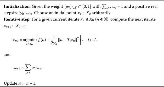

  

  Fixed-point distributed optimization method

• (ii) As the estimate $x_{n,i}$ is the unique minimizer of the constrained subproblem, we can ensure that $x_{n,i}\in X_{0}$ for all $n\in \mathbb {N}$ and $i\in \mathcal {I}$. This means that the sequences $\{x_{n,i}\}_{n\in \mathbb {N}}$, $i\in \mathcal {I}$, are bounded. Furthermore, since the iterate $x_{n}$ belongs to the convex hull of all estimates $x_{n,i}, i\in \mathcal {I}$, the boundedness of the sequence $\{x_{n}\}_{n\in \mathbb {N}}\subset X_{0}$ is guaranteed.

• (iii) Let us compare Algorithm 1 with the existing distributed optimization method. Actually, the method in [23] is based on the fixed-point approximation method and the proximal method like the proposed method. The difference is that, in such a paper, each user i computes

  $$\begin{aligned} y_{n,i}=\mathop{\operatorname{argmin}}_{u\in \mathbb {R}^{k}} \biggl\lbrace f(u)+ \frac{1}{2\gamma _{n}} \Vert u-x_{n} \Vert ^{2} \biggr\rbrace , \end{aligned}$$

  and, subsequently, computes

  $$\begin{aligned} x_{n,i}=\alpha _{n} x_{n} +(1-\alpha _{n})T_{i} y_{n,i}, \end{aligned}$$

  where $\alpha _{n}$ is a positive sequence. Moreover, it can be noted that the weight $\omega _{i}=\frac{1}{m}$ and the constrained set $X_{0}$ are omitted in such a paper. In order to prove the convergence result, the assumption that the sequence $\{y_{n,i}\}_{n\in \mathbb {N}}$ is bounded for all $i\in \mathcal {I}$ is needed in such a paper, whereas in this paper, the boundedness of the generated sequences is neglected.

To get started with the convergence result, we present an important property of the iterates given in Algorithm 1.

Lemma 3.1

Let the sequence $\{x_{n}\} _{n\in \mathbb {N}}\subset X_{0}$ and the stepsize $\{\gamma _{n}\} _{n\in \mathbb {N}}\subset (0,+\infty )$ be given in Algorithm 1. For every $y\in X$ and $n\in \mathbb{N}$, we have

$$\begin{aligned} \Vert x_{n+1}-y \Vert ^{2} \leq {}& \Vert x_{n}-y \Vert ^{2}-\sum_{i\in \mathcal {I}} \omega _{i} \bigl(\rho _{i} \Vert T_{i} x_{n}-x_{n} \Vert ^{2}+ \Vert T_{i}x_{n}-x_{n,i} \Vert ^{2}\bigr) \\ &{}+2\gamma _{n}\sum_{i\in \mathcal {I}}\omega _{i}\bigl(f_{i}(y)-f_{i}(x_{n,i}) \bigr). \end{aligned}$$

Proof

Let $y\in X$ and $n\in \mathbb{N}$ be given. For every $i\in \mathcal {I}$, we note that

$$\begin{aligned} \Vert T_{i}x_{n}-y \Vert ^{2} = \Vert T_{i}x_{n}-x_{n,i} \Vert ^{2}+2\langle T_{i}x_{n}-x_{n,i},x_{n,i}-y \rangle + \Vert x_{n,i}-y \Vert ^{2}. \end{aligned}$$

(5)

By the definition of $x_{n,i}$ and Proposition 2.7, we have

$$\begin{aligned} 0 \in \partial \biggl(f_{i}+\frac{1}{2\gamma _{n}} \Vert \cdot -T_{i}x_{n} \Vert ^{2} \biggr) (x_{n,i})+N_{X_{0}}(x_{n,i}). \end{aligned}$$

Applying Proposition 2.5, we obtain

$$\begin{aligned} 0 \in \partial f_{i}(x_{n,i})+\frac{1}{\gamma _{n}}(x_{n,i}-T_{i}x_{n})+N_{X_{0}}(x_{n,i}), \end{aligned}$$

and then

$$\begin{aligned} \frac{1}{\gamma _{n}}(T_{i}x_{n}-x_{n,i}) \in \partial f_{i}(x_{n,i})+N_{X_{0}}(x_{n,i}). \end{aligned}$$

(6)

By virtue of the above relation (6) and Proposition 2.5, we have, for every $i\in \mathcal {I}$,

$$\begin{aligned} \frac{1}{\gamma _{n}}(T_{i}x_{n}-x_{n,i}) &\in \partial f_{i}(x_{n,i})+ \partial \imath _{X_{0}}(x_{n,i}) \\ &= \partial (f_{i}+\imath _{X_{0}}) (x_{n,i}). \end{aligned}$$

The definitions of subgradient and indicator function of $X_{0}$ yield for every $i\in \mathcal {I}$ that

$$\begin{aligned} \biggl\langle \frac{1}{\gamma _{n}}(T_{i}x_{n}-x_{n,i}),y-x_{n,i} \biggr\rangle &\leq (f_{i}+\imath _{X_{0}}) (y)-(f_{i}+\imath _{X_{0}}) (x_{n,i}) \\ &= f_{i}(y)+\imath _{X_{0}}(y)-f_{i}(x_{n,i})- \imath _{X_{0}}(x_{n,i}) \\ &= f_{i}(y)-f_{i}(x_{n,i}). \end{aligned}$$

(7)

Now, by using equation (5) and inequality (7), we obtain for every $i\in \mathcal {I}$ that

$$\begin{aligned} \Vert x_{n,i}-y \Vert ^{2} \leq \Vert T_{i}x_{n}-y \Vert ^{2}- \Vert T_{i}x_{n}-x_{n,i} \Vert ^{2}+2 \gamma _{n}\bigl(f_{i}(y)-f_{i}(x_{n,i})\bigr). \end{aligned}$$

The strong quasi-nonexpansivity of $T_{i}$ implies for every $i\in \mathcal {I}$ that

$$\begin{aligned} \omega _{i} \Vert x_{n,i}-y \Vert ^{2} \leq{}& \omega _{i} \bigl[ \Vert x_{n}-y \Vert ^{2}- \rho _{i} \Vert T_{i}x_{n}-x_{n} \Vert ^{2} - \Vert T_{i}x_{n}-x_{n,i} \Vert ^{2} \\ &{}+2\gamma _{n}\bigl(f_{i}(y)-f_{i}(x_{n,i}) \bigr)\bigr]. \end{aligned}$$

(8)

By summing up the above inequality for all $i\in \mathcal {I}$ and using the convexity of $\|\cdot \|^{2}$, we obtain that

$$\begin{aligned} \Vert x_{n+1}-y \Vert ^{2} ={}& \biggl\Vert \sum _{i\in \mathcal {I}} \omega _{i} x_{n,i}-y \biggr\Vert ^{2} \\ \leq {}& \sum_{i\in \mathcal {I}} \omega _{i} \Vert x_{n,i}-y \Vert ^{2} \\ \leq {}& \sum_{i\in \mathcal {I}} \omega _{i}\bigl[ \Vert x_{n}-y \Vert ^{2}-\rho _{i} \Vert T_{i}x_{n}-x_{n} \Vert ^{2} - \Vert T_{i}x_{n}-x_{n,i} \Vert ^{2} \\ &{}+2\gamma _{n}\bigl(f_{i}(y)-f_{i}(x_{n,i}) \bigr)\bigr] \\ ={}& \Vert x_{n}-y \Vert ^{2} - \sum _{i\in \mathcal {I}} \omega _{i}\bigl(\rho _{i} \Vert T_{i}x_{n}-x_{n} \Vert ^{2} + \Vert T_{i}x_{n}-x_{n,i} \Vert ^{2}\bigr) \\ &{}+2\gamma _{n}\sum_{i\in \mathcal {I}}\omega _{i}\bigl(f_{i}(y)-f_{i}(x_{n,i}) \bigr), \end{aligned}$$

as desired. □

The following theorem indicates the existence of a convergence subsequence of the generated sequence to the solution set. Note from the above lemma that the sequence $\{\|x_{n}-y\|^{2}\}_{n\in \mathbb {N}}$ is not necessarily decreasing, so we need to divide the proof of the following theorem into two cases.

Theorem 3.2

Let the sequence $\{ x_{n}\} _{n\in \mathbb {N}}\subset X_{0}$ and the stepsize $\{\gamma _{n}\} _{n\in \mathbb {N}}\subset (0,+\infty )$ be given in Algorithm 1. Suppose that $\lim_{n \to +\infty }\gamma _{n} = 0$ and $\sum_{n\in \mathbb {N}}\gamma _{n} = + \infty$. If the operator $T_{i}, i\in \mathcal {I}$, satisfies the DC principle, then the following statements hold:

• (i) There exists a subsequence of the sequence $\{x_{n}\}_{n\in \mathbb{N}}$ that converges to a point $x^{*}$ in $\mathcal{S}$.

• (ii) For each user $i\in \mathcal {I}$, there exists a subsequence of the sequence $\{x_{n,i}\}_{n\in \mathbb{N}}$ that converges to $x^{*}$.

Proof

Since $\{x_{n,i}\}_{n\in \mathbb{N}}$ is a bounded sequence, there exists $M>0$ such that

$$\begin{aligned} \Vert y-x_{n,i} \Vert \leq M_{i}\leq M:=\max _{i\in \mathcal {I}}M_{i} \end{aligned}$$

for every $y\in X$ and for all $i\in \mathcal {I}$. Moreover, since $f_{i}$ is Lipschitz continuous relative to every bounded subset of $\mathbb {R}^{k}$ for all $i\in \mathcal {I}$, there exists ${L}_{i}>0$ such that

$$\begin{aligned} \bigl\vert f_{i}(y)-f_{i}(x_{n,i}) \bigr\vert \leq {L}_{i} \Vert y-x_{n,i} \Vert , \end{aligned}$$

and then

$$\begin{aligned} \sum_{i\in \mathcal {I}} \omega _{i} \bigl(f_{i}(y)-f_{i}(x_{n,i})\bigr)\leq LM, \end{aligned}$$

(9)

where ${L}:=\max_{i\in \mathcal {I}}L_{i}$. By using these two obtained results, the relation in Lemma 3.1 becomes

$$\begin{aligned} \Vert x_{n+1}-y \Vert ^{2} \leq {}& \Vert x_{n}-y \Vert ^{2} \\ &{}-\sum_{i\in \mathcal {I}}\omega _{i}\bigl( \rho _{i} \Vert T_{i}x_{n}-x_{n} \Vert ^{2}+ \Vert T_{i}x_{n}-x_{n,i} \Vert ^{2}\bigr)+2\gamma _{n}{L}M. \end{aligned}$$

(10)

In order to prove the convergence result, we will divide the proof into two cases according to behavior of the sequence $\{\|x_{n}-y\|^{2}\} _{n\in \mathbb{N}}$.

Case 1. Assume that there exists ${n_{0}}\in \mathbb{N}$ such that $\|x_{n+1}-y\|^{2}\leq \|x_{n}-y\|^{2}$ for all $y\in X$ and for all $n\geq n_{0}$. In this case, we have that the sequence $\{\|x_{n}-y\|^{2}\}_{n\in \mathbb{N}}$ is decreasing and bounded from below, hence $\lim_{n\to +\infty }\|x_{n}-y\|^{2}$ exists. Now, we note from (10) that

$$\begin{aligned} \sum_{i\in \mathcal {I}}\omega _{i}\bigl(\rho _{i} \Vert T_{i}x_{n}-x_{n} \Vert ^{2}+ \Vert T_{i}x_{n}-x_{n,i} \Vert ^{2}\bigr) \leq \Vert x_{n}-y \Vert ^{2}- \Vert x_{n+1}-y \Vert ^{2}+2\gamma _{n} LM, \end{aligned}$$

and, by the convergence of $\{\|x_{n}-y\|^{2}\}_{n\in \mathbb{N}}$ and the assumption that $\lim_{n\to +\infty }\gamma _{n}=0$, we obtain that

$$\begin{aligned} \limsup_{n\to +\infty }\sum_{i\in \mathcal {I}}\omega _{i}\bigl(\rho _{i} \Vert T_{i}x_{n}-x_{n} \Vert ^{2}+ \Vert T_{i}x_{n}-x_{n,i} \Vert ^{2}\bigr)\leq 0. \end{aligned}$$

This implies that

$$\begin{aligned} \lim_{n\to +\infty } \Vert T_{i}x_{n}-x_{n} \Vert =\lim_{n\to +\infty } \Vert T_{i}x_{n}-x_{n,i} \Vert =0 \quad\text{for all } i\in \mathcal {I}. \end{aligned}$$

Observing that

$$\begin{aligned} \Vert x_{n}-x_{n,i} \Vert \leq \Vert x_{n}-T_{i}x_{n} \Vert + \Vert T_{i}x_{n}-x_{n,i} \Vert \quad\text{for all } i\in \mathcal {I}, \end{aligned}$$

(11)

it follows that

$$\begin{aligned} \lim_{n\to +\infty } \Vert x_{n}-x_{n,i} \Vert =0\quad \text{for all } i\in \mathcal {I}. \end{aligned}$$

(12)

On the other hand, since the sequences $\{x_{n}\}_{n\in \mathbb{N}}$ and $\{x_{n,i}\}_{n\in \mathbb{N}}, i\in \mathcal {I}$, are bounded, we also have

$$\begin{aligned} \bigl\vert f_{i}(x_{n})-f_{i}(x_{n,i}) \bigr\vert \leq L \Vert x_{n}-x_{n,i} \Vert \quad \text{for all } i \in \mathcal {I}. \end{aligned}$$

Observe that

$$\begin{aligned} f_{i}(y)-f_{i}(x_{n,i})&\leq f_{i}(y)-f_{i}(x_{n})+ \bigl\vert f_{i}(x_{n})-f_{i}(x_{n,i}) \bigr\vert \\ &\leq f_{i}(y)-f_{i}(x_{n})+L \Vert x_{n}-x_{n,i} \Vert \quad\text{for all } i \in \mathcal {I}, \end{aligned}$$

which implies that

$$\begin{aligned} \sum_{i\in \mathcal {I}} \omega _{i} \bigl(f_{i}(y)-f_{i}(x_{n,i}) \bigr) \leq f(y)-f(x_{n})+L\sum_{i\in \mathcal {I}} \omega _{i} \Vert x_{n}-x_{n,i} \Vert . \end{aligned}$$

By applying Lemma 3.1 together with the above relation, we have

$$\begin{aligned} \gamma _{n} \biggl(f(x_{n})-f(y)-L\sum _{i\in \mathcal {I}} \omega _{i} \Vert x_{n}-x_{n,i} \Vert \biggr) \leq \frac{ \Vert x_{n}-y \Vert ^{2}}{2}- \frac{ \Vert x_{n+1}-y \Vert ^{2}}{2}. \end{aligned}$$

(13)

Putting $\beta _{n}:=f(x_{n})-f(y)-L\sum_{i=1}^{m}\omega _{i}\|x_{n}-x_{n,i} \|$ for all $n\geq n_{0}$ and summing up the above inequality (13) for $n=n_{0}$ to infinity yield that

$$\begin{aligned} \sum_{n=n_{0}}^{+\infty } \gamma _{n}\beta _{n}\leq \frac{ \Vert x_{n_{0}}-y \Vert ^{2}}{2}< +\infty. \end{aligned}$$

This implies that

$$\begin{aligned} \sum_{n\in \mathbb {N}}\gamma _{n}\beta _{n}< +\infty. \end{aligned}$$

We next show that $\liminf_{n\to {+\infty }}\beta _{n}\leq 0$. Now, suppose to the contrary that there exist $x\in X,n'\in \mathbb{N}$, and $\alpha >0$ in which $\beta _{n}\geq \alpha$ for all $n\geq n'$. Note that

$$\begin{aligned} {+\infty }=\alpha \sum_{n=n'}^{+\infty } \gamma _{n}\leq \sum_{n=n'}^{+ \infty } \gamma _{n}\beta _{n}< {+\infty }, \end{aligned}$$

which leads to a contradiction. Thus, we have

$$\begin{aligned} \liminf_{n\to {+\infty }} \biggl(f(x_{n})-f(y)-L\sum _{i\in \mathcal {I}} \omega _{i} \Vert x_{n}-x_{n,i} \Vert \biggr)\leq 0 \end{aligned}$$

for all $y\in X$. Since $\lim_{n\to +\infty }\|x_{n}-x_{n,i}\|=0$ for all $i\in \mathcal {I}$, we obtain that $\liminf_{n\to +\infty }f(x_{n})\leq f(y)$. This means that there is a subsequence $\{x_{n_{p}}\}_{p\in \mathbb{N}}$ of $\{x_{n}\}_{n\in \mathbb{N}}$ in which, for every $y\in X$,

$$\begin{aligned} \lim_{p\to +\infty } f(x_{n_{p}})=\liminf _{n\to +\infty } f(x_{n}) \leq f(y). \end{aligned}$$

(14)

Since $\{x_{n_{p}}\}_{p\in \mathbb{N}}$ is a bounded sequence, there exists a subsequence $\{x_{n_{p_{l}}}\}_{l\in \mathbb{N}}$ of $\{x_{n_{p}}\}_{n\in \mathbb{N}}$ such that $\lim_{l\to +\infty }x_{n_{p_{l}}}= x^{*}\in \mathbb{R}^{k}$. We know that $\lim_{l\to +\infty }\|T_{i}x_{n_{p_{l}}}-x_{n_{p_{l}}}\|= 0$ for all $i\in \mathcal {I}$, the DC principle of $T_{i}$ yields that $x^{*}\in \operatorname {Fix}T_{i}$ for all $i\in I$, and hence $x^{*}\in \bigcap_{i\in \mathcal {I}} \operatorname {Fix}T_{i}$. Moreover, since $\{x_{n_{p_{l}}}\}_{l\in \mathbb{N}}\subset X_{0}$ which is a closed set, we also have $x^{*}\in X_{0}$. It follows that $x^{*}\in X$. The continuity of f together with inequality (14) imply that

$$\begin{aligned} f\bigl(x^{*}\bigr)\leq \lim_{l\to +\infty }f(x_{n_{p_{l}}}) \leq f(y), \end{aligned}$$

that is, $x^{*}\in \mathcal{S}$.

Finally, it remains to show that $x_{n_{p}}\to x^{*}\in \mathcal{S}$. By the boundedness of $\{x_{n_{p}}\}_{n\in \mathbb{N}}$, it suffices to show that there is no subsequence $\{x_{n_{p_{r}}}\}_{r\in \mathbb{N}}$ of $\{x_{n_{p}}\}_{n\in \mathbb{N}}$ such that $\lim_{r\to +\infty }x_{n_{p_{r}}}=\bar{x}\in \mathcal{S}$ and $x^{*}\neq \bar{x}$. Indeed, if this is not true, the well-known Opial’s theorem yields

$$\begin{aligned} \lim_{n\to +\infty } \bigl\Vert x_{n}-x^{*} \bigr\Vert =\lim_{l\to +\infty } \bigl\Vert x_{n_{p_{l}}}-x^{*} \bigr\Vert &< \lim_{l\to +\infty } \Vert x_{n_{p_{l}}}-\bar{x} \Vert \\ &= \lim_{n\to +\infty } \Vert x_{n}-\bar{x} \Vert \\ &=\lim_{r\to +\infty } \Vert x_{n_{p_{r}}}-\bar{x} \Vert \\ &< \lim_{r\to +\infty } \bigl\Vert x_{n_{p_{r}}}-x^{*} \bigr\Vert =\lim_{n\to +\infty } \bigl\Vert x_{n}-x^{*} \bigr\Vert , \end{aligned}$$

which leads to a contradiction. Therefore, the sequence $\{x_{n_{p}}\}_{p\in \mathbb{N}}$ converges to a point $x^{*}\in \mathcal{S}$, which proves (i). Moreover, by using (12), we also obtain that $\lim_{p\to +\infty }x_{n_{p},i}=x^{*}\in \mathcal{S}$ for all $i\in \mathcal {I}$, which means that (ii) holds.

Case 2. Assume that there exist a point $y\in X$ and a subsequence $\{x_{n_{j}}\}_{j\in \mathbb{N}}$ of $\{x_{n}\}_{n\in \mathbb{N}}$ such that $\|x_{n_{j}}-y\|^{2}<\|x_{n_{j}+1}-y\|^{2}$ for all $j\in \mathbb {N}$.

Let the sequence $\{\tau (n)\}_{n\geq n_{0}}$ be defined as in Proposition 2.8, we have, for all $n\geq n_{0}$,

$$\begin{aligned} \Vert x_{\tau (n)}-y \Vert ^{2}< \Vert x_{\tau (n)+1}-y \Vert ^{2} \end{aligned}$$

(15)

and

$$\begin{aligned} \Vert x_{n}-y \Vert ^{2}< \Vert x_{\tau (n)+1}-y \Vert ^{2}. \end{aligned}$$

(16)

By applying (10) and (15), we note that

$$\begin{aligned} \sum_{i=1}^{m}\omega _{i}\bigl( \rho _{i} \Vert T_{i}x_{\tau (n)}-x_{\tau (n)} \Vert ^{2}+ \Vert T_{i}x_{\tau (n)}-x_{{\tau (n)},i} \Vert ^{2}\bigr) &\leq a_{\tau (n)}-a_{{ \tau (n)}+1}+2\gamma _{\tau (n)} LM \\ &\leq 2\gamma _{\tau (n)} LM, \end{aligned}$$

and by using the assumption that $\lim_{n \to +\infty }\gamma _{n} = 0$, we obtain

$$\begin{aligned} \limsup_{n\to +\infty }\sum_{i=1}^{m} \omega _{i}\bigl(\rho _{i} \Vert T_{i}x_{ \tau (n)}-x_{\tau (n)} \Vert ^{2}+ \Vert T_{i}x_{\tau (n)}-x_{{\tau (n)},i} \Vert ^{2}\bigr) \leq 0. \end{aligned}$$

Thus, for all $i\in \mathcal {I}$,

$$\begin{aligned} \lim_{n\to +\infty } \Vert T_{i}x_{\tau (n)}-x_{\tau (n)} \Vert =\lim_{n\to + \infty } \Vert T_{i}x_{\tau (n)}-x_{{\tau (n)},i} \Vert =0. \end{aligned}$$

Note that

$$\begin{aligned} \Vert x_{\tau (n)}-x_{{\tau (n)},i} \Vert \leq \Vert x_{\tau (n)}-T_{i}x_{\tau (n)} \Vert + \Vert T_{i}x_{\tau (n)}-x_{{\tau (n)},i} \Vert , \end{aligned}$$

which implies that

$$\begin{aligned} \lim_{n\to +\infty } \Vert x_{\tau (n)}-x_{{\tau (n)},i} \Vert =0 \quad\text{for all } i\in \mathcal {I}. \end{aligned}$$

(17)

Again, by using (13), we have for all $n\geq n_{0}$

$$\begin{aligned} \gamma _{\tau (n)} \Biggl(f(x_{\tau (n)})-f(y)-L\sum _{i=1}^{m} \omega _{i} \Vert x_{\tau (n)}-x_{{\tau (n)},i} \Vert \Biggr) \leq \frac{a_{\tau (n)}}{2}- \frac{a_{{\tau (n)}+1}}{2}, \end{aligned}$$

which together with (15) implies

$$\begin{aligned} f(x_{\tau (n)})-f(y)-L\sum_{i=1}^{m} \omega _{i} \Vert x_{\tau (n)}-x_{{ \tau (n)},i} \Vert \leq 0 \quad\text{for all } n\geq n_{0}. \end{aligned}$$

Subsequently, by using (17) together with the above relation, we obtain that

$$\begin{aligned} \limsup_{n\to +\infty }f(x_{\tau (n)})\leq f(y). \end{aligned}$$

(18)

Thus, there exists a subsequence $\{x_{\tau ({n_{q}})}\}_{q\in \mathbb{N}}$ of $\{x_{\tau (n)}\}_{n\ge n_{0}}$ such that

$$\begin{aligned} \limsup_{q\to +\infty }f(x_{\tau ({n_{q}})})\leq \limsup _{n\to + \infty }f(x_{\tau (n)}). \end{aligned}$$

(19)

Since the sequence $\{x_{\tau (n_{q})}\}_{q\in \mathbb{N}}$ is bounded, there exists a subsequence $\{x_{\tau ({n_{q_{l}}})}\}_{l\in \mathbb{N}}$ of $\{x_{\tau ({n_{q}})}\}_{q\in \mathbb{N}}$ such that $\lim_{l\to +\infty }x_{\tau (n_{q_{l}})}= x^{*}\in \mathbb{R}^{k}$. Moreover, we also have $\lim_{l\to +\infty }\|T_{i}x_{\tau (n_{q_{l}}})-x_{\tau (n_{q_{l}}}) \|= 0$. By the DC principle of $T_{i}, i\in \mathcal {I}$, we have $x^{*}\in \operatorname {Fix}T_{i}$ for all $i\in \mathcal {I}$; consequently, $x^{*}\in \bigcap_{i\in \mathcal {I}} \operatorname {Fix}T_{i}$. Moreover, we also know that $\{x_{\tau (n_{q_{l}})}\}_{l\in \mathbb{N}}\subset X_{0}$, which is a closed set, it follows that $x^{*}\in X_{0}$, and hence $x^{*}\in X$. Invoking (18) and (19), we obtain that

$$\begin{aligned} f\bigl(x^{*}\bigr)\leq \liminf_{l\to +\infty }f(x_{\tau ({n_{q_{l}}})}) \leq \limsup_{l\to +\infty }f(x_{\tau ({n_{q_{l}}})})\leq f(y), \end{aligned}$$

which implies that $x^{*}\in \mathcal{S}$.

By using (17), we note that $\lim_{l\to +\infty }x_{\tau (n_{q_{l}}),i}=x^{*}$ for all $i\in \mathcal {I}$.

Since $\lim_{l\to +\infty }\|x_{\tau (n_{q_{l}})}-x^{*}\|=0$, in view of (16), we note that

$$\begin{aligned} 0\leq \liminf_{l\to +\infty } \bigl\Vert x_{n_{q_{l}}}-x^{*} \bigr\Vert \leq \limsup_{l \to +\infty } \bigl\Vert x_{n_{q_{l}}}-x^{*} \bigr\Vert \leq \limsup_{l\to +\infty } \bigl\Vert x_{ \tau (n_{q_{l}})}-x^{*} \bigr\Vert =0, \end{aligned}$$

which yields that $\lim_{l\to +\infty }x_{n_{q_{l}}}=x^{*}\in \mathcal{S}$. Similarly, we have $\lim_{l\to +\infty }x_{n_{q_{l}},i}=x^{*}\in \mathcal{S}$ for all $i\in \mathcal {I}$. From Cases 1 and 2, there exist a subsequence of $\{x_{n}\}_{n\in \mathbb{N}}$ and $\{x_{n,i}\}_{n\in \mathbb{N}}$ for all $i\in \mathcal {I}$ that converge to a point in $\mathcal{S}$. □

By assuming at least one of the objective functions $f_{i}$ to be strictly convex, we obtain the convergence of the whole sequences as the following theorem.

Theorem 3.3

Let the sequence $\{ x_{n}\} _{n\in \mathbb {N}}\subset X_{0}$ and the stepsize $\{\gamma _{n}\} _{n\in \mathbb {N}}\subset (0,+\infty )$ be given in Algorithm 1. Suppose that $\lim_{n \to +\infty }\gamma _{n} = 0$ and $\sum_{n\in \mathbb {N}}\gamma _{n} = + \infty$. If the operator $T_{i}, i\in \mathcal {I}$, satisfies the DC principle and at least function $f_{i}$ is strictly convex, then the sequences $\{x_{n}\}_{n\in \mathbb{N}}$ and $\{x_{n,i}\}_{n\in \mathbb{N}}, i\in \mathcal {I}$, converge to the unique point solution to problem (4).

Proof

Note that, since the objective function $f:=\sum_{i=1}^{m} f_{i}$ is strictly convex, we have that the solution set to problem (4) consists of at most one point, denoted by $x^{*}$. To this end, we also consider the proof in two cases in the same manner as the lines of the proof of Theorem 3.2.

In case 1, we obtain that there is a subsequence $\{x_{n_{p}}\}_{p\in \mathbb{N}}$ of the sequence $\{x_{n}\}_{n\in \mathbb{N}}$ that converges to a point $x^{*}\in \mathcal{S}$. However, in the context of strict convexity of f, we have $\mathcal{S}=\{x^{*}\}$. These imply that the sequence $\{x_{n}\}_{n\in \mathbb{N}}$ converges to $x^{*}$. Moreover, by using (12), we also obtain that the sequences $\{x_{n,i}\}_{n\in \mathbb{N}}, i\in \mathcal {I}$, also converge to $x^{*}$.

In case 2, we obtain that there is a subsequence $\{x_{\tau (n_{q_{l}})} \}_{l\in \mathbb{N}}$ of $\{x_{\tau (n)}\}_{n\ge n_{0}}$ that converges to $x^{*}$, which yields that the sequence $\{x_{\tau (n)} \}_{n\in \mathbb{N}}$ converges to $x^{*}$, that is, $\lim_{n\to \infty }\|x_{\tau (n)}-x^{*}\|=0$. Since it holds that $\|x_{n}-x^{*}\|\leq \|x_{\tau (n)+1}-x^{*}\|$ for all $n\geq n_{0}$, which implies that

$$\begin{aligned} \limsup_{n\to \infty } \bigl\Vert x_{n}-x^{*} \bigr\Vert \leq \lim_{n\to \infty } \bigl\Vert x_{ \tau (n)+1}-x^{*} \bigr\Vert =0, \end{aligned}$$

which is nothing else than the whole sequence $\{x_{n}\}_{n\in \mathbb{N}}$ converging to $x^{*}$. It is akin as above, we also obtain that the sequences $\{x_{n,i}\}_{n\in \mathbb{N}}, i\in \mathcal {I}$, also converge to $x^{*}$. This completes the proof. □

In the next theorem, we provide an error bound for the feasibility error of iterates per iteration. Actually, we first find the error bound of the weighted averages of distance of the iterates $x_{n}$ to the common fixed point sets.

Theorem 3.4

Let the sequence $\{ x_{n}\} _{n\in \mathbb {N}}\subset X_{0}$ and the stepsize $\{\gamma _{n}\} _{n\in \mathbb {N}}\subset (0,+\infty )$ be given in Algorithm 1. Suppose that $\{\gamma _{n}\}_{n\in \mathbb{N}}$ is a sequence such that $\gamma _{n}=\frac{a}{n^{b}}$, where $a>0$ and $0< b<1$. Then, for every $n\in \mathbb {N}$, we have

$$\begin{aligned} \sum_{i\in \mathcal {I}}\omega _{i} \biggl( \frac{\sum_{k=1}^{n} \Vert T_{i}x_{k}-x_{k} \Vert ^{2}}{n} \biggr) \leq \biggl( \rho ^{-1}d^{2}_{\mathcal{S}}(x_{1})+ \frac{4\rho ^{-1}aLD_{X_{0}}}{1-b} \biggr)\frac{1}{n^{b}}, \end{aligned}$$

where $d_{\mathcal{S}}(x):=\inf_{y\in \mathcal{S}}\|x-y\|$, $D_{X_{0}}:=\max_{x,y\in X_{0}}\|x-y\|<+\infty$, $\rho:=\min_{i\in \mathcal {I}}\rho _{i}$, and ${L}:=\max_{i\in \mathcal {I}}L_{i}$, in which $L_{i}$ is the Lipschitz constant relative to every bounded subset of $\mathbb {R}^{k}$ of each function $f_{i}$.

Proof

Since $\{x_{n,i}\}_{n\in \mathbb{N}}$ is a bounded sequence, there exists $M>0$ such that

$$\begin{aligned} \bigl\Vert P_{\mathcal{S}}(x_{1})-x_{n,i} \bigr\Vert \leq \bigl\Vert P_{\mathcal{S}}(x_{1}) \bigr\Vert + \Vert x_{n,i} \Vert \leq 2D_{X_{0}} \end{aligned}$$

and for all $i\in \mathcal {I}$. Moreover, since $f_{i}$ is Lipschitz continuous relative to every bounded subset of $\mathbb {R}^{k}$, for all $i\in \mathcal {I}$, there exists ${L}_{i}>0$ such that

$$\begin{aligned} \bigl\vert f_{i}\bigl(P_{\mathcal{S}}(x_{1}) \bigr)-f_{i}(x_{n,i}) \bigr\vert \leq {L}_{i} \bigl\Vert P_{\mathcal{S}}(x_{1})-x_{n,i} \bigr\Vert , \end{aligned}$$

and then

$$\begin{aligned} \sum_{i\in \mathcal {I}} \omega _{i} \bigl(f_{i}\bigl(P_{\mathcal{S}}(x_{1}) \bigr)-f_{i}(x_{n,i})\bigr) \leq 2LD_{X_{0}}, \end{aligned}$$

(20)

where ${L}:=\max_{i\in \mathcal {I}}L_{i}$. By invoking the relation in (10), we have, for each $n\in \mathbb{N}$,

$$\begin{aligned} \sum_{i\in \mathcal {I}}\omega _{i}\sum _{k=1}^{n} \bigl(\rho _{i} \Vert T_{i}x_{k}-x_{k} \Vert ^{2}+ \Vert T_{i}x_{k}-x_{k,i} \Vert ^{2} \bigr) \leq \bigl\Vert x_{1}-P_{\mathcal{S}}(x_{1}) \bigr\Vert ^{2}+4LD_{X_{0}}\sum_{k=1}^{n} \gamma _{k}, \end{aligned}$$

which in turn implies that

$$\begin{aligned} \min_{i\in \mathcal {I}}\rho _{i}\sum _{i\in \mathcal {I}}\omega _{i} \biggl( \frac{\sum_{k=1}^{n} \Vert T_{i}x_{k}-x_{k} \Vert ^{2}}{n} \biggr) &\leq \frac{1}{n}\sum_{i\in \mathcal {I}}\omega _{i}\sum_{k=1}^{n} \bigl( \Vert T_{i}x_{k}-x_{k} \Vert ^{2}+ \Vert T_{i}x_{k}-x_{k,i} \Vert ^{2} \bigr) \\ &\leq \frac{d^{2}_{\mathcal{S}}(x_{1})}{n}+\frac{4LD_{X_{0}}}{n}\sum_{k=1}^{n} \gamma _{k}, \end{aligned}$$

and then

$$\begin{aligned} \sum_{i\in \mathcal {I}}\omega _{i} \biggl( \frac{\sum_{k=1}^{n} \Vert T_{i}x_{k}-x_{k} \Vert ^{2}}{n} \biggr) \leq \frac{\rho ^{-1}d^{2}_{\mathcal{S}}(x_{1})}{n}+ \frac{4\rho ^{-1}LD_{X_{0}}}{n}\sum _{k=1}^{n}\gamma _{k}. \end{aligned}$$

Now, let us note that

$$\begin{aligned} \frac{1}{n}\sum_{k=1}^{n}\gamma _{k}=\frac{1}{n}\sum_{k=1}^{n} \frac{a}{k^{b}}\leq \frac{a}{n} \int _{t=1}^{t=n}\frac{1}{t^{b}}\,dt= \frac{a}{n} \biggl[\frac{n^{1-b}}{1-b}-\frac{1}{1-b} \biggr]\leq \frac{a}{1-b}\frac{1}{n^{b}}, \end{aligned}$$

which implies that

$$\begin{aligned} \sum_{i\in \mathcal {I}}\omega _{i} \biggl( \frac{\sum_{k=1}^{n} \Vert T_{i}x_{k}-x_{k} \Vert ^{2}}{n} \biggr) \leq \biggl(\rho ^{-1}d^{2}_{\mathcal{S}}(x_{1})+ \frac{4\rho ^{-1}aLD_{X_{0}}}{1-b} \biggr)\frac{1}{n^{b}}, \end{aligned}$$

as desired. □

The above theorem provides an upper bound on the rate of convergence in which the weighted average sequence $\sum_{i\in \mathcal {I}}\omega _{i} ( \frac{\sum_{k=1}^{n}\|T_{i}x_{k}-x_{k}\|^{2}}{n} )$ of the distance of the sequence $x_{n}$ to the fixed point set $\operatorname {Fix}T_{i}$ converges to 0. It can be seen that the weighted average of the distance is bounded above by a constant factor of $\frac{1}{n^{b}}$, where n is the iteration index and $0< b<1$. In this situation, we can also say that the distance converges to 0 with a rate of $\mathcal{O} (\frac{1}{n^{b}} )$. Moreover, if the weight is identical, that is, $\omega _{i}=1/m$, we obtain the error bound

$$\begin{aligned} \sum_{i\in \mathcal {I}} \biggl( \frac{\sum_{k=1}^{n} \Vert T_{i}x_{k}-x_{k} \Vert ^{2}}{n} \biggr) \leq \biggl( \rho ^{-1}d^{2}_{\mathcal{S}}(x_{1})+ \frac{4\rho ^{-1}aLD_{X_{0}}}{1-b} \biggr)\frac{m}{n^{b}}. \end{aligned}$$

4 Numerical example

In this section, we present a numerical example for solving the minimal distance to given points over a finite number of half-space constraints with box constraint.

Actually, let $a_{i}\in \mathbb{R}^{k}$, $c_{i}\in \mathbb{R}^{k}$, and $b_{i}\geq 0$ be given for all $i=1,2,\ldots,m$, we consider the following minimization problem:

$$\begin{aligned} \begin{aligned} &\mathrm{minimize } \quad \sum _{i=1}^{m} \frac{1}{2} \Vert x-c_{i} \Vert ^{2}, \\ &\mathrm{subject\ to}\quad \langle a_{i},x\rangle \leq b_{i}, i=1,2, \ldots,m, \text{ and $ x\in [u,v]^{k}$,} \end{aligned} \end{aligned}$$

(21)

where $u,v\in \mathbb{R}$ with $u\leq v$. Note that the function $f_{i}:=\frac{1}{2}\|\cdot -c_{i}\|^{2}$ is strictly convex, the constrained set $C_{i}:=\{x\in \mathbb{R}^{k}:\langle a_{i},x\rangle \leq b_{i}\}, i=1,2, \ldots,m$, and the box $X_{0}:=[u,v]^{k}$ are nonempty closed and convex sets. By putting $T_{i}=P_{C_{i}}$, for all $i=1,2,\ldots,m$, we have $T_{i}$ is strongly quasi-nonexpansive and satisfies the DC principle with $\mathrm{Fix} T_{i}=C_{i}$. Thus, the considered problem (21) is nothing else than the particular situation of problem (4), and the sequence generated by Algorithm 1 can be applied for solving the problem.

Observe that Algorithm 1 requires the computation of estimate $x_{n,i}$ for all $i=1,2,\ldots,m$, which is a solution of the minimization problem

$$\begin{aligned} x_{n,i}= \mathop{\operatorname{argmin}}_{u\in X_{0}} \biggl\lbrace f_{i}(u)+ \frac{1}{2\gamma _{n}} \Vert u-T_{i}x_{n} \Vert ^{2} \biggr\rbrace ,\quad i=1,2, \ldots,m. \end{aligned}$$

Of course, the solution cannot be computed explicitly in a closed-form expression. In this situation, we need to solve the following strongly convex optimization problem:

$$\begin{aligned} \begin{aligned}& \mathrm{minimize }\quad \frac{1}{2} \Vert u-c_{i} \Vert ^{2}+ \frac{1}{2\gamma _{n}} \Vert u-P_{C_{i}}x_{n} \Vert ^{2}, \\ &\mathrm{subject\ to}\quad u\in X_{0}. \end{aligned} \end{aligned}$$

Note that the objective function $\frac{1}{2} \|u-c_{i}\|^{2}+\frac{1}{2\gamma _{n}}\|u-P_{C_{i}}x_{n} \|^{2}$ is strongly convex function with modulus $1+\frac{1}{\gamma _{n}}$ and Lipschitz continuous gradient with Lipschitz constant $1+\frac{1}{\gamma _{n}}$. In our experiment, we basically make use of the classical gradient projection method by performing the inner loop: pick an arbitrary initial point $y_{1}\in X_{0}$ and compute

$$\begin{aligned} y_{l+1}=P_{X_{0}} \biggl(y_{l}-\alpha _{l} \biggl[(y_{l}-c_{i})+ \frac{1}{\gamma _{n}}\bigl(y_{l}-P_{C_{i}}x_{n} \bigr) \biggr] \biggr)\quad \forall l\in \mathbb {N}, \end{aligned}$$

where $\alpha _{l}$ is a positive stepsize.

All the experiments were performed under MATLAB 9.9 (R2020b) running on a personal laptop with an AMD Ryzen 7 4800H with Radeon Graphics 2.90 GHz processor and 8GB memory. All CPU times are given in seconds. We generate vectors $a_{i}$ and $c_{i}$ in $\mathbb{R}^{k}$ by uniformly distributed random generating between $(-1,1)$. We choose the box constraint with boundaries $u=0$ and $v=1$. We choose the starting point for every inner loop to be a vector whose coordinates are uniformly distributed randomly chosen from the interval $(0,1)$. An example of a sequence $\{x_{n}\}_{n\in \mathbb {N}}$ generated by Algorithm 1 and its behavior in the simple case of $k=2$ and $m=10$, all $b_{i}=0, i=1,2,\ldots,m$, the stopping criterion for inner loop is 1000 iterations, and the initial point $x_{1}=(1,0.7)^{\top }$ are illustrated in Fig. 1.

Figure 1

Behavior of a sequence $\{x_{n}\}_{n\in \mathbb {N}}$ generated by Algorithm 1

In Fig. 1, we observe from both upper figures that the values of iterates $x_{n}$ and all $x_{n,i}$ for all $i=1,\ldots,10$ converge to the same point, which is coherent with the assertions in Theorem 3.3. Moreover, we can see from the lower left that the feasibility error $\sum_{i\in \mathcal {I}} ( \frac{\sum_{k=1}^{n}\|T_{i}x_{k}-x_{k}\|^{2}}{n} )$ is bounded by the error bound $(\rho ^{-1}d^{2}_{\mathcal{S}}(x_{1})+ \frac{4\rho ^{-1}aLD_{X_{0}}}{1-b} )\frac{m}{n^{b}}$, with $a=1,b=0.9$, which conforms to the result in Theorem 3.4. For the lower right, we present the convergence behavior of the sequence $\{x_{n}\}_{n\in \mathbb {N}}$ which is converging to the solution point $(0,0)^{\top }$ of the minimizing distance to the reference points $c_{i}$ (blue dots).

In the next experiment, we consider behavior of the sequence $\{x_{n}\}_{n\in \mathbb {N}}$ generated by Algorithm 1 for various problem’s dimensions for two stopping criteria of inner loops. We generate vectors $a_{i}$ and $c_{i}$ as above, and $b_{i}$ is normally distributed randomly chosen in $(1,2)$. We choose the initial point to be a vector whose all coordinates are uniformly distributed randomly chosen in $(0, 1)$. We manually choose the best choices of the involved stepsizes, that is, $\gamma _{n}=1.8/n$ and $\alpha _{l}=1.6/l$. We terminate Algorithm 1 by the stopping criteria $\frac{\|x_{n+1}-x_{n}\|}{\|x_{n}\|+1}\leq 10^{-6}$. We performed 10 independent tests for any collections of dimensions $k=10, 20, 50$, and 100 and the number of nodes $m=3, 5, 10, 20$, 50, and 100. The results are presented in Table 1, where the average number of iterations and the average computational runtime for any collection of k and m are presented.

Table 1 Behavior of Algorithm 1 for different dimensions (k) and different number of nodes (m)

We have presented in Table 1 the number of iterations (k) (#(Iters)), the computational time (Time) in seconds, where the number of inner iterations (#(Inner)) is 1000 and 10,000 when the stopping criteria of Algorithm 1 were met. It can be observed that larger k and m require a larger number of iterations and computational runtime. Moreover, for the case when $m=3, 5, 10$, and 20, we observe that the number of inner iterations 1000 is sufficient enough for the convergence of Algorithm 1 with less than about 10 times comparing with the case when the number of inner iterations is $10{,}000$ in computational runtime. Nevertheless, for the very large dimension with $k=100$ and $m=50, 100$, the number of inner iterations 1000 may not be sufficient for the convergence of Algorithm 1.

References

Bauschke, H.H., Combettes, P.L.: Convex Analysis and Monotone Operator Theory in Hilbert Spaces, 2nd edn. Springer, New York (2017)
Beck, A.: First-Ordered Methods in Optimization. SIAM, Philadelphia (2017)
Bnouhachem, A.: A descent SQP alternating direction method for minimizing the sum of three convex functions. J. Nonlinear Var. Anal. 4, 469–482 (2020)
Bnouhachem, A., Qin, X.: An inertial proximal Peaceman–Rachford splitting method with SQP regularization for convex programming. J. Nonlinear Funct. Anal. (2020). https://doi.org/10.23952/jnfa.2020.50
Cauchy, A.L.: Methode generale pour la resolution des systemes d’equations simultanees. C. R. Acad. Sci. Paris 25, 536–538 (1847)
Cegielski, A.: Iterative Methods for Fixed Point Problems in Hilbert Spaces. Lecture Notes in Mathematics, vol. 2057. Springer, Berlin (2012)
Gibali, A., Shehu, Y.: An efficient iterative method for finding common fixed point and variational inequalities in Hilbert spaces. Optimization 68(1), 13–32 (2019)
Iiduka, H.: Iterative algorithm for triple-hierarchical constrained nonconvex optimization problem and its application to network bandwidth allocation. SIAM J. Optim. 22(3), 862–878 (2012)
Iiduka, H.: Fixed point optimization algorithms for distributed optimization in networked systems. SIAM J. Optim. 23(1), 1–26 (2013)
Iiduka, H.: Proximal point algorithms for nonsmooth convex optimization with fixed point constraints. Eur. J. Oper. Res. 253(2), 503–513 (2016)
Iiduka, H.: Distributed optimization for network resource allocation with nonsmooth utility functions. IEEE Trans. Control Netw. Syst. 6(4), 1354–1365 (2019)
Iiduka, H.: Stochastic fixed point optimization algorithm for classifier ensemble. IEEE Trans. Cybern. 50(10), 4370–4380 (2020)
Iiduka, H., Hishinuma, K.: Acceleration method combining broadcast and incremental distributed optimization algorithms. SIAM J. Optim. 24(4), 1840–1863 (2014)
Iiduka, H., Uchida, M.: Fixed point optimization algorithms for network bandwidth allocation problems with compoundable constraints. IEEE Commun. Lett. 15(6), 596–598 (2011)
Iiduka, H., Yamada, I.: Computational method for solving a stochastic linearquadratic control problem given an unsolvable stochastic algebraic Riccati equation. SIAM J. Control Optim. 50, 2173–2192 (2012)
Maingé, P.E.: Strong convergence of projected subgradient methods for nonsmooth and nonstrictly convex minimization. Set-Valued Anal. 16, 899–912 (2008)
Martinet, B.: Determination approchee d’un point fixe d’une application pseudocontractante. C. R. Acad. Sci. Paris 274A, 163–165 (1972)
Nimana, N.: A fixed-point subgradient splitting method for solving constrained convex optimization problems. Symmetry 12(3), 377 (2020)
Ono, S., Yamada, I.: Hierarchical convex optimization with primal-dual splitting. IEEE Trans. Signal Process. 63, 373–388 (2015)
Prangprakhon, M., Nimana, N.: Extrapolated sequential constraint method for variational inequality over the intersection of fixed-point sets. Numer. Algorithms 88, 1051–1075 (2021)
Rockafellar, R.T.: Extension of Fenchel’s duality theorem for convex functions. Duke Math. J. 33(1), 81–89 (1966)
Rosen, J.B.: The gradient projection method for nonlinear programming, part 2: nonlinear constraints. SIAM J. Appl. Math. 9, 514–553 (1961)
Sakurai, K., Jimba, T., Iiduka, H.: Iterative methods for parallel convex optimization with fixed point constraints. J. Nonlinear Var. Anal. 3(2), 115–126 (2019)
Shehu, Y., Ogbuisi, F.U.: Convergence analysis for proximal split feasibility problems and fixed point problems. J. Appl. Math. Comput. 48(1–2), 221–239 (2015)
Shimizu, K., Hishinuma, K., Iiduka, H.: Parallel computing proximal method for nonsmooth convex optimization with fixed point constraints of quasi-nonexpansive mappings. Appl. Set-Valued Anal. Optim. 2, 1–17 (2020)
Slavakis, K., Yamada, I.: Robust wideband beamforming by the hybrid steepest descent method. IEEE Trans. Signal Process. 55, 4511–4522 (2007)
Yamada, I.: The hybrid steepest descent method for the variational inequality problem over the intersection of fixed point sets of nonexpansive mappings. In: Butnariu, D., Censor, Y., Reich, S. (eds.) Inherently Parallel Algorithms in Feasibility and Optimization and Their Applications, pp. 473–504. Elsevier, Amsterdam (2001)
Yamada, I., Yukawa, M., Yamagishi, M.: Minimizing the Moreau envelope of nonsmooth convex functions over the fixed point set of certain quasi-nonexpansive mappings. In: Bauschke, H.H., Burachik, R.S., Combettes, P.L., Elser, V., Luke, D.R., Wolkowicz, H. (eds.) Fixed-Point Algorithms for Inverse Problems in Science and Engineering, pp. 345–390. Springer, New York (2011)
Acknowledgements
The authors are thankful to the Editor, Prof. Jen-Chih Yao, and two anonymous referees for comments and remarks which improved the quality and presentation of the paper.
Authors’ information
Not applicable.
Funding
N. Ekkarntrong was partially supported by the young researcher development project of Khon Kaen University. T. Arunrat was partially supported by the development and promotion of science and technology talent project (DPST). N. Nimana was partially supported by Thailand Science Research and Innovation under the project IRN62W0007.
Author information
Authors and Affiliations
Contributions
All authors contributed equally. All authors read and approved the final manuscript.
Corresponding author
Ethics declarations
Competing interests
The authors declare that they have no competing interests.
Rights and permissions
Open Access This article is licensed under a Creative Commons Attribution 4.0 International License, which permits use, sharing, adaptation, distribution and reproduction in any medium or format, as long as you give appropriate credit to the original author(s) and the source, provide a link to the Creative Commons licence, and indicate if changes were made. The images or other third party material in this article are included in the article’s Creative Commons licence, unless indicated otherwise in a credit line to the material. If material is not included in the article’s Creative Commons licence and your intended use is not permitted by statutory regulation or exceeds the permitted use, you will need to obtain permission directly from the copyright holder. To view a copy of this licence, visit http://creativecommons.org/licenses/by/4.0/.
About this article
Cite this article
Ekkarntrong, N., Arunrat, T. & Nimana, N. Convergence of a distributed method for minimizing sum of convex functions with fixed point constraints. J Inequal Appl 2021, 197 (2021). https://doi.org/10.1186/s13660-021-02734-4
Received:
Accepted:
Published:
DOI: https://doi.org/10.1186/s13660-021-02734-4