Strong consistency rates for the estimators in a heteroscedastic EV model with missing responses

Abstract

This article is concerned with the semi-parametric error-in-variables (EV) model with missing responses: $y_{i}= \xi _{i}\beta +g(t_{i})+\epsilon _{i}$, $x_{i}= \xi _{i}+\mu _{i}$, where $\epsilon _{i}=\sigma _{i}e_{i}$ is heteroscedastic, $f(u_{i})=\sigma ^{2}_{i}$, $y_{i}$ are the response variables missing at random, the design points $(\xi _{i},t_{i},u_{i})$ are known and non-random, β is an unknown parameter, $g(\cdot )$ and $f(\cdot )$ are functions defined on closed interval $[0,1]$, and the $\xi _{i}$ are the potential variables observed with measurement errors $\mu _{i}$, $e_{i}$ are random errors. Under appropriate conditions, we study the strong consistent rates for the estimators of β, $g(\cdot )$ and $f(\cdot )$. Finite sample behavior of the estimators is investigated via simulations.

1 Introduction

Consider the following semi-parametric error-in-variables (EV) model:

$$ \textstyle\begin{cases} y_{i}= \xi _{i}\beta +g(t_{i})+\epsilon _{i}, \\ x_{i}=\xi _{i}+\mu _{i}, \end{cases} $$

(1.1)

where $\epsilon _{i}=\sigma _{i}e_{i}$, $\sigma ^{2}_{i}=f(u_{i})$, $y_{i}$ are the response variables, $(\xi _{i},t_{i},u_{i})$ are design points, $\xi _{i}$ are the potential variables observed with measurement errors $\mu _{i}$, $E\mu _{i}=0$, $e_{i}$ are random errors with $Ee_{i}=0$ and $Ee_{i}^{2}=1$, β is an unknown parameter, $g(\cdot )$ and $f(\cdot )$ are functions defined on closed interval $[0,1]$. In model (1.1), there exists a function $h(\cdot )$ defined on closed interval $[0,1]$ satisfying

$$ \xi _{i}=h(t_{i})+v_{i}, $$

(1.2)

where $v_{i}$ are also design points.

Model (1.1) includes many special forms which were studied by many scholars in recent years for complete data. When $\mu _{i}\equiv 0$, it reduces to the general semi-parametric model, which was first introduced by Engle et al. [5] to study the effect of weather on electricity demand.

In many applications, however, there often exist covariate measurement errors. For example, it has been well documented in the literature that covariates such as blood pressure, urinary sodium chloride level, and exposure to pollutants are often subject to measurement errors, and covariate measurement errors may cause difficulties and complications in conducting statistical analysis. So EV models are somewhat more practical than ordinary regression models. When $g(\cdot )\equiv 0$, the model (1.1) reduces to the usual linear EV model. Fan et al. [6] discussed the strong consistency and asymptotic normality for the estimators of the ordinary least-square estimators. Further discussions can be found in Miao et al. [15], Miao and Liu [14], Liu and Chen [13] and so on. Model (1.1) has also been investigated by some authors. Cui and Li [4] derived the asymptotic distributions for the estimators of β, $g(\cdot )$ and error variance. Hu et al. [10] derived the asymptotic normality for the estimators of the parametric and nonparametric components; Zhou et al. [22] discussed the inference process for asymptotic distribution of estimators.

In the literature on the semi-parametric model and the EV model, scholars mainly study the situation of complete data, but in practical applications, they often encounter the situation of incomplete data. Incomplete data includes missing data, truncated data and censored data. Among them, missing data is the most common. In practical application, variables may be lost due to design or happenstance. For example, the responses $y_{i}$ may be very expensive to measure and only part of the $y_{i}$ are available. Another example is that the $y_{i}$ represent the responses to a set of questions and some sampled individuals refuse to supply the desired information. Actually, missing of responses is very common in opinion polls, market research surveys, mail enquiries, social-economic investigations, and so on. Xu et al. [19] investigated the problem of testing nonparametric function and proposed two bias-corrected test statistics based on the quadratic conditional moment method. Yang and Xia [20] derived the asymptotically normal distribution for the restricted estimator of the parametric component. Wei and Mei [18] defined an empirical likelihood-based statistic and error-prone covariates and proved that its limiting distribution is a chi-square distribution.

Missing data includes completely random loss (MCAR), random missing (MAR) and nonrandom missing (NMAR). In this paper, we choose model (1.1) and assume that $y_{i}$ is missing at random (MAR). Therefore, we obtain a random incomplete data sequence ${(y_{i},\delta _{i},\xi _{i},t_{i})}$. The MAR assumption implies that $\delta _{i}$ and $y_{i}$ are conditionally independent given $\xi _{i}$ and $t_{i}$. That is, $P(\delta _{i}=1|y_{i},\xi _{i},t_{i})=P(\delta _{i}=1|\xi _{i},t_{i})$. The MAR is a common assumption for statistical analysis with missing data and is reasonable in many practical situations; see Little and Rubin [12].

When people face the loss of data, one method is to delete data with missing values. Another method is interpolation, which is based on the analysis of fully observed data and uses predicted or average values to interpolate the missing part of the data. In regression problems, commonly used imputation approaches include linear regression imputation by Healy and Westmacott [9], nonparametric kernel regression imputation by Cheng [3], semi-parametric regression imputation by Wang et al. [16], and by Wang and Sun [17]. This paper extends the methods to the estimation of β and $g(\cdot )$ under the semi-parametric EV model (1.1). We use two methods to estimate β and $g(\cdot )$ with missing responses and study the strong consistent rates for the estimators of β and $g(\cdot )$, according to $f(\cdot )$ being known or unknown.

The paper is organized as follows. In Sect. 2, we list some assumptions. The main results are given in Sect. 3. Simulation study is presented in Sect.s 4. Some preliminary lemmas are stated in Sect. 5. Proofs of the main results are provided in Sect. 6.

2 Assumptions

In this section, we list some assumptions, which will be used in the theorems below.

• (A0) Let $\{e_{i}, 1\leq i\leq n\}$, $\{\mu _{i}, 1\leq i\leq n\}$ and $\{\delta _{i}, 1\leq i\leq n\}$ be independent random variables satisfying

  • (i) $Ee_{i}=0$, $E\mu _{i}=0$, $Ee_{i}^{2}=1$, $E\mu _{i}^{2}=\varXi _{\mu }^{2}>0$.

  • (ii) $\sup_{i}E|e_{i}|^{\gamma _{1}}<\infty$, $\sup_{i}E| \mu _{i}|^{\gamma _{2}}<\infty$ from some ${\gamma _{1}}>8/3$, ${\gamma _{2}}>4$.

  • (iii) $\{e_{i}, 1\leq i\leq n\}$, $\{\mu _{i}, 1\leq i\leq n\}$ and $\{\delta _{i}, 1\leq i\leq n\}$ are independent of each other.

• (A1) Let $\{v_{i}, 1\leq i\leq n\}$ in (1.2) be a sequence satisfying $0<\varSigma _{i}<\infty$ for $i=0,1,2,3$.

  • (i) $\lim_{n\to \infty }n^{-1}\sum_{i=1}^{n}v^{2}_{i}=\varSigma _{0}, \lim_{n\to \infty }n^{-1}\sum_{i=1}^{n}\delta _{i}v^{2}_{i}=\varSigma _{1}$$a.s$.

  • (ii) $\lim_{n\to \infty }n^{-1}\sum_{i=1}^{n}\sigma ^{-2}_{i}v^{2}_{i}= \varSigma _{2}, \lim_{n\to \infty }n^{-1}\sum_{i=1}^{n}\sigma ^{-2}_{i} \delta _{i}v^{2}_{i}=\varSigma _{3}$$a.s$.

  • (iii) $\lim_{n\to \infty }\sup_{n}(\sqrt{n}\log n)^{-1}\max_{1\leq m \leq n}|\sum_{i=1}^{m}\delta _{j_{i}}v_{j_{i}}|<\infty$$a.s$., where $\{j_{1},j_{2},\ldots,j_{n}\}$ is a permutation of $(1,2,\ldots,n)$.

  • (iv) $\max_{1\leq i\leq n}|v_{i}|=O(n^{1/8})$.

• (A2)

  • (i) $0< m\leq \min_{1\leq i\leq n}f(u_{i})\leq \max_{1\leq i\leq n}f(u_{i}) \leq M<\infty$.

  • (ii) $f(\cdot )$, $g(\cdot )$, $h(\cdot )$ satisfy the first-order Lipschitz condition on a closed interval $[0, 1]$.

• (A3) Let $W_{nj}^{c}(t)$$(1\leq j\leq n)$ be weight functions defined on $[0, 1]$ and satisfying

  • (i) $\max_{1\leq j\leq n}\sum_{i=1}^{n}\delta _{j}W_{nj}^{c}(t_{i}) = O(1)$ a.s.

  • (ii) $\sup_{t\in [0, 1]}\sum_{j=1}^{n}\delta _{j}W_{nj}^{c}(t)I( |t - t_{j} | > a\cdot n^{-1/4})=o(n^{-1/4})$ a.s. for any $a>0$.

  • (iii) $\sup_{t\in [0, 1]}\max_{1\leq j\leq n}W_{nj}^{c}(t) = o(n^{-1/2} \log ^{-1}n)$ a.s.

• (A4) Let $W_{nj}(t)$$(1\leq j\leq n)$ be weight functions defined on $[0, 1]$ and satisfying

  • (i) $\max_{1\leq j\leq n}\sum_{i=1}^{n}W_{nj}(t_{i}) = O(1)$.

  • (ii) $\sup_{t\in [0, 1]}\sum_{j=1}^{n}W_{nj}(t)I( |t - t_{j} | > a \cdot n^{-1/4}) = o(n^{-1/4})$ for any $a>0$.

  • (iii) $\sup_{t\in [0, 1]}\max_{1\leq j\leq n}W_{nj}(t)=o(n^{-1/2}\log ^{-1}n)$.

• (A5) Let $\hat{W}_{nj}^{c}(u)\ (1\leq j\leq n)$ be weight functions defined on $[0, 1]$ and satisfying (A3).

Remark 2.1

Assumptions (A0)–(A5) are standard regularity conditions and they are used commonly in the literature; see Gao et al. [7], Härdle et al. [8] and Chen [2].

3 Main results

3.1 Estimation without considering heteroscedasticity

For model (1.1) without heteroscedasticity, firstly, one deletes all the missing data. Then one can get the model $\delta _{i}y_{i}= \delta _{i}\xi _{i}\beta +\delta _{i}g(t_{i})+ \delta _{i}\epsilon _{i}$. If $\xi _{i}$ can be observed, we can apply the least-square estimation method to estimate the parameter β. If β is known, using the complete data ${(\delta _{i}y_{i},\delta _{i}x_{i},\delta _{i}t_{i}),1\leq i\leq n}$, the estimator of $g(\cdot )$, given β, is

$$\begin{aligned} g_{n}^{*}(t, \beta )=\sum _{j=1}^{n}W_{nj}^{c}(t) ( \delta _{j}y_{j}- \delta _{j}x_{j} \beta ). \end{aligned}$$

(3.1)

Then under this condition of the semi-parametric EV model, Liang et al. [11] improved the least-square estimator (LSE) on the basis of the usual partially linear model, and employed the estimator of parameter β to minimize the following formula:

$$\begin{aligned} SS(\beta )=\sum_{i=1}^{n}\delta _{i} \bigl\{ \bigl[y_{i}-x_{i}\beta -g^{*}_{n}(t_{i}, \beta ) \bigr]^{2}- \varXi _{\mu }^{2}\beta ^{2} \bigr\} . \end{aligned}$$

Therefore, one can get the LSE of β

$$\begin{aligned} \hat{\beta }_{c} = \Biggl[\sum _{i=1}^{n}\delta _{i}\bigl( \tilde{x_{i}^{c}}^{2}- \varXi _{\mu }^{2} \bigr) \Biggr]^{-1}\sum_{i=1}^{n} \delta _{i}\tilde{x_{i}^{c}} \tilde{y_{i}^{c}}, \end{aligned}$$

(3.2)

where $\tilde{x_{i}^{c}}=x_{i}-\sum_{j=1}^{n}\delta _{j}W_{nj}^{c}(t_{i})x_{j}$, $\tilde{y_{i}^{c}}=y_{i}-\sum_{j=1}^{n}\delta _{j}W_{nj}^{c}(t_{i})y_{j}$.

Using $\hat{\beta }_{c}$, we define the following the estimators of $g(\cdot )$:

$$\begin{aligned} \hat{g}_{n}^{c}(t) = \sum _{j=1}^{n}\delta _{j}W_{nj}^{c}(t) (y_{j}-x_{j} \hat{\beta }_{c}). \end{aligned}$$

(3.3)

Apparently, the estimators $\beta _{c}$ and $g_{n}^{c}(t)$ are formed without taking all sample information into consideration. Hence, in order to make up for the missing data, we imply an imputation method from Wang and Sun [17], and let

$$\begin{aligned} U_{i}^{I}=\delta _{i}y_{i}+(1-\delta _{i})\bigl[x_{i} \hat{\beta }_{c}+ \hat{g}_{n}^{c}(t_{i}) \bigr]. \end{aligned}$$

(3.4)

Therefore, using complete data ${(U_{i}^{I},x_{i},t_{i}),1\leq i\leq n}$, similar to (3.2) and (3.3), one can get other estimators for β and $g(\cdot )$, that is,

$$\begin{aligned} \hat{\beta }_{I}= \Biggl[\sum _{i=1}^{n}\bigl(\tilde{x}_{i}^{2}- \delta _{i} \varXi _{\mu }^{2}\bigr) \Biggr]^{-1}\sum_{i=1}^{n} \tilde{x}_{i}\tilde{U}_{i}^{I}. \end{aligned}$$

(3.5)

Using $\hat{\beta }_{I}$, we define the following the estimators of $g(\cdot )$:

$$\begin{aligned} \hat{g}_{n}^{I}(t)=\sum _{j=1}^{n}W_{nj}(t) \bigl(U_{j}^{I}-x_{j} \hat{\beta }_{I}\bigr), \end{aligned}$$

(3.6)

where $\tilde{U}_{i}^{I}={U}_{i}^{I}-\sum_{j=1}^{n}W_{nj}(t_{i}){U}_{j}^{I}$, $\tilde{x}_{i}=x_{i}-\sum_{j=1}^{n}W_{nj}(t_{i})x_{j}$.

3.2 Estimation when $\sigma _{i}^{2}=f(u_{i})$ are known

When the errors are heteroscedastic, we consider two different cases according to $f(\cdot )$. If $\sigma _{i}^{2}=f(u_{i})$ are known, then β̂ is modified to be the weighted least-square estimator (WLSE)

$$\begin{aligned} \hat{\beta }_{W_{1}} = \Biggl[\sum _{i=1}^{n}\sigma _{i}^{-2} \delta _{i}\bigl( \tilde{x_{i}^{c}}^{2}- \varXi _{\mu }^{2}\bigr) \Biggr]^{-1}\sum _{i=1}^{n}\sigma _{i}^{-2} \delta _{i}\tilde{x_{i}^{c}}\tilde{y_{i}^{c}}. \end{aligned}$$

(3.7)

Using $\hat{\beta }_{W_{1}}$, we define the following the estimators of $g(\cdot )$:

$$\begin{aligned} \hat{g}_{n}^{W_{1}}(t) = \sum_{j=1}^{n}\delta _{j}W_{nj}^{c}(t) (y_{j}-x_{j} \hat{\beta }_{W_{1}}). \end{aligned}$$

(3.8)

Then similar to (3.4) one can make up for the missing data and let

$$\begin{aligned} U_{i}^{I_{1}}=\delta _{i}y_{i}+(1-\delta _{i})\bigl[x_{i} \hat{\beta }_{W_{1}}+ \hat{g}_{n}^{W_{1}}(t_{i}) \bigr]. \end{aligned}$$

(3.9)

Therefore, using complete data ${(U_{i}^{I_{1}},x_{i},t_{i}),1\leq i\leq n}$, similar to (3.4)–(3.5), one can get other estimators for β and $g(\cdot )$, that is,

$$\begin{aligned} \hat{\beta }_{I_{1}}= \Biggl[\sum _{i=1}^{n}\sigma _{i}^{-2}\bigl( \tilde{x}_{i}^{2}- \delta _{i}\varXi _{\mu }^{2}\bigr) \Biggr]^{-1}\sum _{i=1}^{n}\sigma _{i}^{-2} \tilde{x}_{i}\tilde{U}_{i}^{I_{1}}. \end{aligned}$$

(3.10)

Using $\hat{\beta }_{I_{1}}$, we define the following the estimators of $g(\cdot )$:

$$\begin{aligned} \hat{g}_{n}^{I_{1}}(t)=\sum _{j=1}^{n}W_{nj}(t) \bigl(U_{j}^{I_{1}}-x_{j} \hat{\beta }_{I_{1}}\bigr), \end{aligned}$$

(3.11)

where $\tilde{U}_{i}^{I_{1}}={U}_{i}^{I_{1}}-\sum_{j=1}^{n}W_{nj}(t_{i}){U}_{j}^{I_{1}}$, $\tilde{x}_{i}=x_{i}-\sum_{j=1}^{n}W_{nj}(t_{i})x_{j}$.

Therefore, we have the following results.

Theorem 3.1

Suppose that (A0), (A1)(i), (ii), (iii), (A2)–(A3) are satisfied. For every$t\in [0, 1]$, we have

• (a) $\hat{\beta }_{W_{1}} - \beta = o(n^{-\frac{1}{4}})\textit{ a.s.}$

• (b) $\hat{g}_{n}^{W_{1}}(t) -g(t) = o(n^{-\frac{1}{4}})\textit{ a.s.}$

Theorem 3.2

Suppose that (A0), (A1)(i), (ii), (iii), (A2)–(A4) are satisfied. For every$t\in [0, 1]$, we have

• (a) $\hat{\beta }_{I_{1}} - \beta = o(n^{-\frac{1}{4}})\textit{ a.s.}$

• (b) $\hat{g}_{n}^{I_{1}}(t) - g(t) = o(n^{-\frac{1}{4}})\textit{ a.s.}$

3.3 Estimation when $\sigma _{i}^{2}=f(u_{i})$ are unknown

We address the case that the $\sigma _{i}^{2}=f(u_{i})$ are unknown and must be estimated. Note that, when $Ee^{2}_{i}=1$, we have $E[y_{i}-\xi _{i}\beta -g(t_{i})]^{2}=f(u_{i})$. So, the estimator of $f(u_{i})$ can be defined by

$$\begin{aligned} \hat{f}_{n}(u_{i})=\sum _{j=1}^{n}\delta _{j} \hat{W}_{nj}^{c}(u_{i}) \bigl( \tilde{y}_{j}^{c}-\tilde{x}_{j}^{c}\hat{ \beta }_{c}\bigr)^{2}-\varXi _{\mu }^{2} \hat{\beta }_{c}^{2}. \end{aligned}$$

(3.12)

For the sake of convenience, we assume that $\min_{1\leq i\leq n}\hat{f}_{n}(u_{i})>0$. Then we can define a nonparametric estimator of $\sigma _{i}^{2}$, $\hat{\sigma }_{ni}^{2}=\hat{f}_{n}(u_{i})$. Consequently, the WLSE of β is

$$\begin{aligned} \hat{\beta }_{W_{2}} = \Biggl[\sum _{i=1}^{n} \hat{\sigma }_{ni}^{-2} \delta _{i}\bigl(\tilde{x_{i}^{c}}^{2}- \varXi _{\mu }^{2}\bigr) \Biggr]^{-1}\sum _{i=1}^{n} \hat{\sigma }_{ni}^{-2} \delta _{i}\tilde{x_{i}^{c}} \tilde{y_{i}^{c}}. \end{aligned}$$

(3.13)

Using $\hat{\beta }_{W_{2}}$, we define the following estimators of $g(\cdot )$:

$$\begin{aligned} \hat{g}_{n}^{W_{2}}(t) = \sum_{j=1}^{n}\delta _{j}W_{nj}^{c}(t) (y_{j}-x_{j} \hat{\beta }_{W_{2}}). \end{aligned}$$

(3.14)

Similarly, one can make up for the missing data and let

$$\begin{aligned} U_{i}^{I_{2}}=\delta _{i}y_{i}+(1-\delta _{i})\bigl[x_{i} \hat{\beta }_{W_{2}}+ \hat{g}_{n}^{W_{2}}(t_{i}) \bigr]. \end{aligned}$$

(3.15)

Therefore, using complete data ${(U_{i}^{I_{2}},x_{i},t_{i}),1\leq i\leq n}$, one can get other estimators for β and $g(\cdot )$, that is,

$$\begin{aligned} \hat{\beta }_{I_{2}}= \Biggl[\sum _{i=1}^{n} \hat{\sigma }_{ni}^{-2} \bigl( \tilde{x}_{i}^{2}-\delta _{i}\varXi _{\mu }^{2}\bigr) \Biggr]^{-1}\sum _{i=1}^{n} \hat{\sigma }_{ni}^{-2} \tilde{x}_{i}\tilde{U}_{i}^{I_{2}}. \end{aligned}$$

(3.16)

Using $\hat{\beta }_{I_{2}}$, we define the following the estimators of $g(\cdot )$:

$$\begin{aligned} \hat{g}_{n}^{I_{2}}(t)= \sum_{j=1}^{n}W_{nj}(t) \bigl(U_{j}^{I_{2}}-x_{j} \hat{\beta }_{I_{2}} \bigr), \end{aligned}$$

(3.17)

where $\tilde{U}_{i}^{I_{2}}={U}_{i}^{I_{2}}-\sum_{j=1}^{n}W_{nj}(t_{i}){U}_{j}^{I_{2}}$, $\hat{\sigma }_{ni}^{2}=\hat{f}_{n}(u_{i})$.

Therefore, we have the following results.

Theorem 3.3

Suppose that (A0)–(A3), (A5) are satisfied with$\gamma _{1}>16/3$and$\gamma _{2}>16/3$in (A0). For every$u\in [0, 1]$, we have$\hat{f}_{n}(u)-f(u)=o(n^{-1/4})\textit{ a.s.}$

Theorem 3.4

Suppose that (A0)–(A3), (A5) are satisfied with$\gamma _{1}>16/3$and$\gamma _{2}>16/3$in (A0). For every$t\in [0, 1]$, we have

• (a) $\hat{\beta }_{W_{2}} - \beta = o(n^{-\frac{1}{4}})\textit{ a.s.}$

• (b) $\hat{g}_{n}^{W_{2}}(t) -g(t) = o(n^{-\frac{1}{4}})\textit{ a.s.}$

Theorem 3.5

Suppose that (A0)–(A5) are satisfied with$\gamma _{1}>16/3$and$\gamma _{2}>16/3$in (A0). For every$t\in [0, 1]$, we have

• (a) $\hat{\beta }_{I_{2}} - \beta = o(n^{-\frac{1}{4}})\textit{ a.s.}$

• (b) $\hat{g}_{n}^{I_{2}}(t) - g(t) = o(n^{-\frac{1}{4}})\textit{ a.s.}$

4 Simulation study

In this section, we carry out a simulation to study the finite sample performance of the proposed estimators. In particular:

• (1) we compare the performance of the estimators $\hat{\beta }_{W_{1}}$, $\hat{\beta }_{I_{1}}$, $\hat{\beta }_{W_{2}}$ and $\hat{\beta }_{I_{2}}$ by their mean squared errors (MSE), also, we compare the performance of the estimators $\hat{g}_{n}^{W_{1}}(\cdot )$, $\hat{g}_{n}^{I_{1}}(\cdot )$, $\hat{g}_{n}^{W_{2}}(\cdot )$ and $\hat{g}_{n}^{I_{2}}(\cdot )$ by their global mean squared errors (GMSE);

• (2) we give the boxplots for the estimators of β and $g(t_{n/2})$;

• (3) we give the fitting figure for the estimators of $g(\cdot )$.

Observations are generated from

$$ \textstyle\begin{cases} y_{i}= \xi _{i}\beta +g(t_{i})+\epsilon _{i}, \\ x_{i}= \xi _{i}+\mu _{i}, \end{cases} $$

(4.1)

where $\beta =1$, $g(t)=\sin (2\pi t)$, $\epsilon _{i}=\sigma _{i}e_{i}$, $\sigma ^{2}_{i}=f(u_{i})$, $f(u)=[1+0.5\cos (2\pi u)]^{2}$, $t_{i}=(i-0.5)/n$, $u_{i}= (i-1)/n$ and $\xi _{i}=t_{i}^{2}+v_{i}$. {$v_{i}, 1\leq i\leq n$} is an i.i.d. $N(0, 1)$ sequence. $\{\mu _{i}, 1\leq i\leq n\}$ is an i.i.d. $N(0, 0.2^{2})$ sequence. {$e_{i}, 1\leq i\leq n$} is an i.i.d. $N(0, 1)$ sequence. {$v_{i}, 1\leq i\leq n$}, $\{\mu _{i}, 1\leq i\leq n\}$ and {$e_{i}, 1\leq i\leq n$} are independent. $d_{i}$ is a $B(1, 1-p)$ sequence where the missing probability $p=0.1, 0.25, 0.5$. For the proposed estimators, the weight functions are taken as

$$\begin{aligned} W_{ni}^{c}(t)&= \frac{K((t-t_{i})/h_{n})}{\sum_{j=1}^{n}\delta _{j}K((t-t_{j})/h_{n})},\qquad W_{ni}(t)= \frac{K((t-t_{i})/b_{n})}{\sum_{j=1}^{n}K((t-t_{j})/b_{n})}, \\ \hat{W}_{ni}^{c}(u)&= \frac{K((u-u_{i})/l_{n})}{\sum_{j=1}^{n}\delta _{j}K((u-u_{j})/l_{n})}, \end{aligned}$$

where is $K(\cdot )$ a Gaussian kernel function, $h_{n}$, $b_{n}$, $l_{n}$ are bandwidth sequences.

4.1 Compare the estimators for β and $g(\cdot )$

Because otherwise there would be too much computation, we have to take a small sample size for convenience of the simulation. We generate the observed data with sample size n=50, 100 and 200 from the model above. The MSE of the estimators for β based on $M=100$ replications are defined as

$$ \mbox{MSE}(\hat{\beta })=\frac{1}{M}\sum_{l=1}^{M} \bigl[\hat{\beta }(l)- \beta \bigr]^{2}, $$

where $\hat{\beta }(l)$ is the lth estimator of β. The GMSE of the estimators for $g(\cdot )$ are defined as

$$ \mbox{GMSE}(\hat{g})=\frac{1}{Mn}\sum_{l=1}^{M} \sum_{k=1}^{n} \bigl[ \hat{g}(t_{k}, l)-g(t_{k}) \bigr]^{2}, $$

where $\hat{g}(t_{k}, l)$ is the lth estimator of $g(t_{k})$.

It is well known that an important issue is the selection of an appropriate bandwidth sequence. The common methods are grid point and cross-validation. Here we use the grid point method to select optimal bandwidths. The bandwidth sequences $h_{n}$, $b_{n}$, $l_{n}$ are taken uniformly over 50 points with step length of 0.02 on the closed interval $[0,1]$. Then we calculate the MSE for the estimators of β and the GMSE for the estimators $g(\cdot )$ for each $(h_{n},b_{n},l_{n})$ and select optimal bandwidths to minimize the MSE for the estimators of β and the GMSE for the estimators $g(\cdot )$. The MSE or GMSE for the estimators are reported in Tables 1–2. On the other hand, we give the boxplots for the estimators of β and $g(t_{n/2})$ with $n=50, 100, 200$ and $p=0.25$.

Table 1 The MSE for the estimators of β

Table 2 The GMSE for the estimators of $g(\cdot )$ and $f(\cdot )$

From Tables 1–2 and Fig. 1, it can be seen that:

• (i) For every fixed n and p, the MSE of $\hat{\beta }_{I_{1}}$ and $\hat{\beta }_{I_{2}}$ are smaller than that of $\hat{\beta }_{W_{1}}$ and $\hat{\beta }_{W_{2}}$, the GMSE of $\hat{g}_{n}^{I_{1}}(\cdot )$ and $\hat{g}_{n}^{I_{2}}(\cdot )$ are smaller than that of $\hat{g}_{n}^{W_{1}}(\cdot )$ and $\hat{g}_{n}^{W_{2}}(\cdot )$. It shows that the interpolation method is more effective than the delection method.

• (ii) For every fixed n and p, the MSE of $\hat{\beta }_{W_{2}}$ and $\hat{\beta }_{I_{2}}$ are very close to that of $\hat{\beta }_{W_{1}}$ and $\hat{\beta }_{I_{1}}$, the GMSE of $\hat{g}_{n}^{W_{2}}(\cdot )$ and $\hat{g}_{n}^{I_{2}}(\cdot )$ are close to that of $\hat{g}_{n}^{W_{1}}(\cdot )$ and $\hat{g}_{n}^{I_{2}}(\cdot )$.

• (iii) For every fixed n, the MSE for the estimators of β and the GMSE for the estimators of $g(\cdot )$ increase as the increasing of p.

• (iv) For every fixed p, the MSE for the estimators of β and the GMSE for the estimators of $g(\cdot )$ all decrease as the increasing of n.

• (v) Fig. 1 shows that the variances of the estimators decrease on increasing of sample size n.

  Figure 1

  

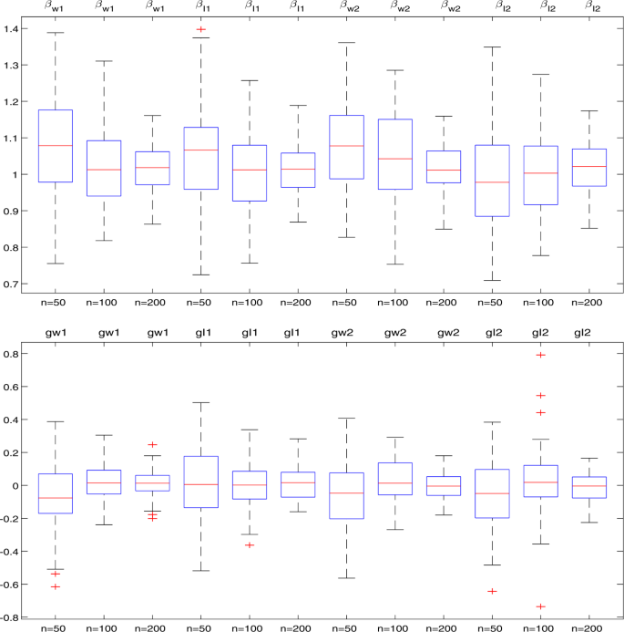
  $p=0.25$ and $n=50$, 100, 200,The boxplots for the estimators of β and $g(\cdot )$

• (vi) The simulation results are consistent with the theoretical results.

4.2 The fitting figure for the estimators of $g(\cdot )$

In this section, we give the fitting figure of $\hat{g}_{n}^{I_{1}}(\cdot )$ and $\hat{g}_{n}^{I_{2}}(\cdot )$ with $p=0.25$. From Figs. 2–3, one can see that

• (i) for every fixed n, the graph for the estimators of $g(\cdot )$ is very close to $g(\cdot )$;

• (ii) for every fixed n, the graph of $\hat{g}_{n}^{I_{1}}(\cdot )$ is very close to $\hat{g}_{n}^{I_{2}}(\cdot )$;

• (iii) the fitting effect is better on the increase of n;

• (iv) when n reaches 200, the fitting effect is ideal;

• (v) the simulation results are consistent with the theoretical results.

Figure 2

$p=0.25$, $n=50$, 100 and 200, the fitting figure for $\hat{g}_{n}^{I_{1}}$

Figure 3

$p=0.25$, $n=50$, 100 and 200, the fitting figure for $\hat{g}_{n}^{I_{2}}$

5 Preliminary lemmas

In the sequel, let $C, C_{1}, C_{2},\ldots$ be some finite positive constants, whose values are unimportant and may change. Now, we introduce several lemmas, which will be used in the proof of the main results.

Lemma 5.1

(Baek and Liang [1], Lemma 3.1)

Let$\alpha > 2$, $e_{1},\ldots,e_{n}$be independent random variables with$Ee_{i}=0$. Assume that$\{a_{ni}, 1\leq i\leq n, n\geq 1\}$is a triangular array of numbers with$\max_{1\leq i\leq n}|a_{ni}| = O(n^{-1/2})$and$\sum_{i=1}^{n}a_{ni}^{2} = o(n^{-2/\alpha }(logn)^{-1})$. If$\sup_{i}E|e_{i}|^{\gamma }< \infty$for some$\gamma >2\alpha /(\alpha -1)$, then

$$ \sum_{i=1}^{n}a_{ni}e_{i} = o\bigl(n^{-1/\alpha }\bigr) \quad\textit{a.s.} $$

Lemma 5.2

(Härdle et al. [8], Lemma A.3)

Let$V_{1}, \ldots, V_{n}$be independent random variables with$EV_{i}=0$, and$\sup_{1\leq j\leq n}E|V_{j}|^{r}\leq C<\infty (r>2)$. Assume that$\{a_{ki}, k, i=1, \ldots, n\}$is a sequence of numbers such that$\sup_{1\leq i, k\leq n}|a_{ki}|=O(n^{-p_{1}})$for some$0< p_{1}<1$and$\sum_{j=1}^{n}a_{ji}=O(n^{p_{2}})$for$p_{2}\geq \max (0, 2/r-p_{1})$. Then

$$ \max_{1\leq i\leq n} \Biggl\vert \sum_{k=1}^{n}a_{ki}V_{k} \Biggr\vert =O\bigl(n^{-s} \log n\bigr)\quad\textit{a.s. for } s=(p_{1}-p_{2})/2. $$

Following the proof line of Lemma 4.7 in Zhang and Liang [21], one can verify the following two lemmas.

Lemma 5.3

• (a) Let$\tilde{A}_{i}=A(t_{i})-\sum_{j=1}^{n}W_{nj}(t_{i})A(t_{j})$, where$A(\cdot )=g(\cdot )$or$h(\cdot )$. Let$\tilde{A}^{c}_{i}=A(t_{i})-\sum_{j=1}^{n}\delta _{j}W_{nj}^{c}(t_{i})A(t_{j})$, where$A(\cdot )=g(\cdot )$or$h(\cdot )$. Then (A0)–(A4) imply that$\max_{1\leq i\leq n}|\tilde{A}_{i}|=o(n^{-1/4})$and$\max_{1\leq i\leq n}|\tilde{A}^{c}_{i}|=o(n^{-1/4})$a.s.

• (b) (A0)–(A4) imply that$n^{-1}\sum_{i=1}^{n}\tilde{\xi }_{i}^{2}\to \varSigma _{0}$, $\sum_{i=1}^{n}|\tilde{\xi }_{i}|\leq C_{1}n$, $n^{-1}\sum_{i=1}^{n}\delta _{i}(\tilde{\xi }_{i}^{c})^{2}\to \varSigma _{1}$a.s. and$\sum_{i=1}^{n}|\delta _{i}\tilde{\xi }_{i}^{c}|\leq C_{2}n$a.s.

• (c) (A0)–(A4) imply that$n^{-1}\sum_{i=1}^{n}\sigma _{i}^{-2}\tilde{\xi }_{i}^{2}\to \varSigma _{2}$, $\sum_{i=1}^{n}|\sigma _{i}^{-2}\tilde{\xi }_{i}|\leq C_{3}n$, $n^{-1}\sum_{i=1}^{n}\sigma _{i}^{-2}\delta _{i}(\tilde{\xi }_{i}^{c})^{2} \to \varSigma _{3}$a.s. and$\sum_{i=1}^{n}|\sigma _{i}^{-2}\delta _{i}\tilde{\xi }_{i}^{c}| \leq C_{4}n$a.s.

• (d) (A0)–(A4) imply that$\max_{1\leq i\leq n}|\tilde{\xi }_{i}|=O(n^{1/8})$and$\max_{1\leq i\leq n}|\tilde{\xi }_{i}^{c}|=O(n^{1/8})$a.s.

• (e) (A0)–(A4) imply that$\max_{1\leq i\leq n}|\sigma _{i}^{-2}\tilde{\xi }_{i}|=O(n^{1/8})$and$\max_{1\leq i\leq n}|\sigma _{i}^{-2}\tilde{\xi }_{i}^{c}|=O(n^{1/8})$a.s.

Lemma 5.4

• (a) Suppose that (A0)–(A4) are satisfied. Then one can deduce that

  $$ \max_{1\leq i\leq n} \bigl\vert \hat{g}_{n}^{W_{1}}(t_{i})-g(t_{i}) \bigr\vert =o\bigl(n^{- \frac{1}{4}}\bigr) \quad\textit{a.s.} $$

• (b) Suppose that (A0)–(A4) are satisfied. Then one can deduce that

  $$ \max_{1\leq i\leq n} \bigl\vert \hat{g}_{n}^{W_{2}}(t_{i})-g(t_{i}) \bigr\vert =o\bigl(n^{- \frac{1}{4}}\bigr) \quad\textit{a.s.} $$

One can easily get Lemma 5.3 by (A0)–(A4). The proof of Lemma 5.4 is analogous to the proof of Theorem 3.1(b) and Theorem 3.2(b).

6 Proof of main results

Now, we introduce some notations which will be used in the proofs below.

$$\begin{aligned} &\tilde{\xi _{i}^{c}}=\xi _{i}-\sum _{j=1}^{n}\delta _{j}W_{nj}^{c}(t_{i}) \xi _{j},\qquad \tilde{\mu _{i}^{c}} = \mu _{i}-\sum_{j=1}^{n}\delta _{j}W_{nj}^{c}(t_{i}) \mu _{j},\\ & \tilde{g^{c}_{i}}=g(t_{i})-\sum _{j=1}^{n}\delta _{j}W_{nj}^{c}(t_{i})g(t_{j}), \\ &\tilde{\epsilon ^{c}_{i}}=\epsilon _{i}-\sum _{j=1}^{n}\delta _{j}W_{nj}^{c}(t_{i}) \epsilon _{j}, \qquad \tilde{\xi }_{i}=\xi _{i}-\sum _{j=1}^{n}W_{nj}(t_{i}) \xi _{j}, \qquad\tilde{\mu }_{i} = \mu _{i}-\sum _{j=1}^{n}W_{nj}(t_{i}) \mu _{j}, \\ &\tilde{g_{i}}=g(t_{i})-\sum _{j=1}^{n}W_{nj}(t_{i})g(t_{j}),\qquad \tilde{\epsilon }_{i} = \epsilon _{i}-\sum _{j=1}^{n}W_{nj}(t_{i}) \epsilon _{j},\qquad S_{n}^{2} = \sum _{i=1}^{n}\sigma _{i}^{-2} \tilde{ \xi }_{i}^{2}, \\ &S_{1n}^{2}=\sum_{i=1}^{n} \sigma _{i}^{-2}\bigl(\delta _{i} \tilde{x_{i}^{c}}^{2}-\delta _{i}\varXi _{\mu }^{2}\bigr),\qquad S_{2n}^{2} = \sum _{i=1}^{n}\sigma _{i}^{-2} \bigl(\tilde{x}_{i}^{2}-\delta _{i}\varXi _{\mu }^{2}\bigr). \end{aligned}$$

Proof of Theorem 3.1(a)

From (3.7), one can write

$$\begin{aligned} \hat{\beta }_{W_{1}}-\beta ={}& S_{1n}^{-2} \Biggl[\sum_{i=1}^{n} \sigma _{i}^{-2} \delta _{i}\bigl(\tilde{\xi _{i}^{c}} + \tilde{\mu _{i}^{c}}\bigr) \tilde{y_{i}^{c}} - \sum_{i=1}^{n} \sigma _{i}^{-2}\delta _{i} \bigl(\bigl( \tilde{\xi _{i}^{c}} + \tilde{\mu _{i}^{c}} \bigr)^{2}-\varXi _{\mu }^{2} \bigr)\beta \Biggr] \\ ={}& S_{1n}^{-2} \Biggl[\sum_{i=1}^{n} \sigma _{i}^{-2}\delta _{i}\bigl( \tilde{\xi _{i}^{c}} + \tilde{\mu _{i}^{c}}\bigr) \bigl(\tilde{g_{i}^{c}} + \tilde{\epsilon _{i}^{c}} - \tilde{\mu _{i}^{c}}\beta \bigr) + \sum_{i=1}^{n} \sigma _{i}^{-2}\delta _{i}\varXi _{\mu }^{2} \beta \Biggr] \\ ={}& S_{1n}^{-2} \Biggl\{ \sum_{i=1}^{n} \sigma _{i}^{-2}\delta _{i} \tilde{\xi _{i}^{c}}(\epsilon _{i}-\mu _{i}\beta ) + \sum_{i=1}^{n} \sigma _{i}^{-2}\delta _{i}\mu _{i}\epsilon _{i} - \sum_{i=1}^{n} \sigma _{i}^{-2}\delta _{i}\bigl(\mu _{i}^{2} - \varXi _{\mu }^{2}\bigr)\beta \\ &{} + \sum_{i=1}^{n}\sigma _{i}^{-2}\delta _{i}\tilde{\xi _{i}^{c}} \tilde{g_{i}^{c}} + \sum _{i=1}^{n}\sigma _{i}^{-2} \delta _{i} \tilde{\mu _{i}^{c}} \tilde{g_{i}^{c}} - \sum_{i=1}^{n} \sum_{j=1}^{n} \sigma _{i}^{-2} \delta _{i}\delta _{j}W_{nj}^{c}(t_{i}) \tilde{\xi _{i}^{c}}\epsilon _{j} \\ &{} -\sum_{i=1}^{n}\sum _{j=1}^{n}\sigma _{i}^{-2}\delta _{i}\delta _{j}W_{nj}^{c}(t_{i}) \epsilon _{i}\mu _{j} -\sum_{i=1}^{n} \sum_{j=1}^{n}\sigma _{i}^{-2} \delta _{i}\delta _{j}W_{nj}^{c}(t_{i}) \mu _{i}\epsilon _{j} \\ &{} +\sum_{i=1}^{n}\sum _{j=1}^{n}\sigma _{i}^{-2}\delta _{i}\delta _{j}W_{nj}^{c}(t_{i}) \tilde{\xi _{i}^{c}}\mu _{j}\beta +2\sum _{i=1}^{n}\sum_{j=1}^{n} \sigma _{i}^{-2}\delta _{i}\delta _{j}W_{nj}^{c}(t_{i})\mu _{i}\mu _{j} \beta \\ &{} +\sum_{i=1}^{n}\sum _{j=1}^{n}\sum_{k=1}^{n} \sigma _{i}^{-2} \delta _{i}\delta _{j} \delta _{k}W_{nj}^{c}(t_{i})W_{nk}^{c}(t_{i}) \mu _{j}\epsilon _{k} \\ &{} -\sum_{i=1}^{n}\sum _{j=1}^{n}\sum_{k=1}^{n} \sigma _{i}^{-2} \delta _{i}\delta _{j} \delta _{k}W_{nj}^{c}(t_{i})W_{nk}^{c}(t_{i}) \mu _{j}\mu _{k}\beta \Biggr\} \\ :={}& S_{1n}^{-2}\sum_{k=1}^{12}A_{kn}. \end{aligned}$$

(6.1)

Thus, to prove $\hat{\beta }_{W_{1}}-\beta =o(n^{-1/4}) \text{ a.s.}$, we only need to verify that $S_{1n}^{-2}\leq Cn^{-1} \text{ a.s.}$ and $n^{-1}A_{kn}=o(n^{-1/4}) \text{ a.s.}$ for $k=1,2,\ldots,12$.

Step 1. We prove $S_{1n}^{-2}\leq Cn^{-1} \text{ a.s.}$ Note that

$$\begin{aligned} S_{1n}^{2}={}&\sum_{i=1}^{n} \sigma _{i}^{-2}\delta _{i}\bigl( \tilde{x_{i}^{c}}^{2}-\varXi _{\mu }^{2} \bigr)= \sum_{i=1}^{n} \bigl[\sigma _{i}^{-2} \delta _{i}\bigl(\tilde{\xi }_{i}^{c}+\tilde{\mu }_{i}^{c} \bigr)^{2}-\sigma _{i}^{-2} \delta _{i} \varXi _{\mu }^{2} \bigr] \\ = {}&\sum_{i=1}^{n} \Biggl\{ \sigma _{i}^{-2}\delta _{i} \Biggl[ \tilde{\xi }_{i}^{c}+\mu _{i}-\sum _{j=1}^{n}\delta _{j}W_{n_{j}}^{c}(t_{i}) \mu _{j} \Biggr]^{2}-\sigma _{i}^{-2} \delta _{i}\varXi _{\mu }^{2} \Biggr\} \\ ={}& \sum_{i=1}^{n}\sigma _{i}^{-2}\delta _{i}\bigl(\tilde{\xi }_{i}^{c}\bigr)^{2}+ \sum _{i=1}^{n}\sigma _{i}^{-2}\delta _{i}\bigl(\mu _{i}^{2}-\varXi _{\mu }^{2}\bigr)+ \sum_{i=1}^{n} \sigma _{i}^{-2}\delta _{i} \Biggl[\sum _{j=1}^{n} \delta _{j}W_{nj}^{c}(t_{i}) \mu _{j} \Biggr]^{2} \\ &{} +2\sum_{i=1}^{n}\sigma _{i}^{-2}\delta _{i}\tilde{\xi }_{i}^{c} \mu _{i}-2\sum _{i=1}^{n}\sigma _{i}^{-2}\delta _{i}\tilde{\xi }_{i}^{c} \sum _{j=1}^{n}\delta _{j}W_{nj}^{c}(t_{i}) \mu _{j} -2\sum_{i=1}^{n} \sigma _{i}^{-2}\delta _{i}\mu _{i}\sum _{j=1}^{n} \delta _{j}W_{nj}^{c}(t_{i}) \mu _{j} \\ :={}& B_{1n}+B_{2n}+B_{3n}+B_{4n}+B_{5n}+B_{6n}. \end{aligned}$$

By Lemma 5.3(c), we have $n^{-1}B_{1n}\to \varSigma _{1} \text{ a.s.}$ Next, we verify that $B_{kn}=o(B_{1n})=o(n) \text{ a.s.}$ for $k=2,3,\ldots,6$. Applying (A0), taking $r>2$, $p_{1}=1/2$, $p_{2}=1/2$ in Lemma 5.2, we have

$$\begin{aligned} \sum_{i=1}^{n} (\zeta _{i} - E\zeta _{i} ) =n^{\frac{1}{2}}\cdot \sum _{i=1}^{n}n^{-\frac{1}{2}} (\zeta _{i} - E\zeta _{i} ) = O\bigl(n^{ \frac{1}{2}}\log n \bigr)=o(n) \quad\text{a.s.}, \end{aligned}$$

(6.2)

where $\zeta _{i}$ are independent random variables satisfying $E\zeta _{i}=0$ and $\sup_{1\leq i\leq n}E|\zeta _{i}|^{r}$ <∞. Therefore, we obtain $B_{2n}=O(n^{1/2}\log n)=o(n)$ a.s. from (A0) and (6.2). On the other hand, taking $\alpha =4$, $\gamma >8/3$ in Lemma 5.1, we have

$$\begin{aligned} \max_{1\leq i\leq n} \Biggl\vert \sum_{j=1}^{n}\delta _{j}W_{nj}^{c}(t_{i}) \zeta _{j} \Biggr\vert =o\bigl(n^{-{\frac{1}{4}}}\bigr) \quad\text{a.s.},\qquad \max_{1\leq { i}\leq { n}} \Biggl\vert \sum_{ j=1}^{ n}{ W_{nj}(t_{i}) \zeta _{j}} \Biggr\vert ={ o} \bigl({ n}^{-{\frac{1}{4}}}\bigr) \quad\text{a.s.}, \end{aligned}$$

(6.3)

where the $\zeta _{i}$ are independent random variables satisfying $E\zeta _{i}=0$ and $\sup_{1\leq i\leq n}E|\zeta _{i}|^{\gamma }$ <∞, for some $\gamma >8/3$. It also holds if one replace $W_{nj}^{c}(t_{i})$ with $\hat{W}_{nj}^{c}(u_{i})$. Meanwhile, by (A0) and Lemma 5.2, taking $r=p>2$, $p_{1}=1/4$, $p_{2}=3/4$ in Lemma 5.2, one can also deduce that

$$\begin{aligned} \vert B_{4n} \vert =2n^{{\frac{1}{4}}}\cdot \Biggl\vert \sum_{i=1}^{n} n^{-{ \frac{1}{4}}}\sigma _{i}^{-2}\delta _{i}\tilde{ \xi _{i}^{c}}\mu _{i} \Biggr\vert =O \bigl(n^{\frac{1}{2}}\log n\bigr)=o(n)\quad \text{a.s.} \end{aligned}$$

(6.4)

Note that, from Lemma 5.3, (6.2) and (6.3), we have

$$\begin{aligned} \vert B_{3n} \vert \leq {}&\sum _{i=1}^{n} \bigl\vert \sigma _{i}^{-2} \delta _{i} \bigr\vert \cdot \max_{1\leq i\leq n} \Biggl\vert \sum_{j=1}^{n}\delta _{j}W_{nj}^{c}(t_{i}) \mu _{j} \Biggr\vert ^{2}=o\bigl(n^{\frac{1}{2}}\bigr)\quad \text{a.s.}, \end{aligned}$$

(6.5)

$$\begin{aligned} \vert B_{5n} \vert \leq {}&2\sum _{i=1}^{n} \bigl\vert \sigma _{i}^{-2} \delta _{i} \tilde{\xi }_{i}^{c} \bigr\vert \cdot \max_{1\leq i\leq n} \Biggl\vert \sum _{j=1}^{n} \delta _{j}W_{nj}^{c}(t_{i}) \mu _{j} \Biggr\vert =o\bigl(n^{\frac{3}{4}}\bigr)\quad\text{a.s.}, \end{aligned}$$

(6.6)

$$\begin{aligned} \vert B_{6n} \vert \leq {}&2 \Biggl[\sum _{i=1}^{n}\bigl( \bigl\vert \sigma _{i}^{-2}\delta _{i} \mu _{i} \bigr\vert -E \bigl\vert \sigma _{i}^{-2}\delta _{i} \mu _{i} \bigr\vert \bigr) +\sum_{i=1}^{n}E \bigl\vert \sigma _{i}^{-2}\delta _{i}\mu _{i} \bigr\vert \Biggr]\cdot \max_{1\leq i\leq n} \Biggl\vert \sum_{j=1}^{n}\delta _{j}W_{nj}^{c}(t_{i})\mu _{j} \Biggr\vert \\ ={}&o\bigl(n^{\frac{3}{4}}\bigr) \quad\text{a.s.} \end{aligned}$$

(6.7)

Therefore, for (6.2)–(6.7), one can deduce that $S_{1n}^{2}=B_{1n}+o(n)=B_{1n}+o(B_{1n})$ a.s., which yields

$$ \lim_{n\to \infty }\frac{B_{1n}}{S_{1n}^{2}}=\lim_{n\to \infty } \frac{B_{1n}}{B_{1n}+o(B_{1n})}=1\quad \text{a.s.} $$

Therefore, by Lemma 5.3(b), we get $S_{1n}^{-2}\leq Cn^{-1} \text{ a.s.}$

Step 2. We verify that $n^{-1}A_{kn} = o(n^{-1/4}) \text{ a.s.}$ for $k=1,2,\ldots,12$. From (A0), we find $\{\eta _{i} = \epsilon _{i} - \mu _{i}\beta, 1\leq i\leq n\}$ are sequences of independent random variables with $E\eta _{i}=0$, $\sup_{i}E |\eta _{i} |^{p} \leq C\sup_{i}E |\epsilon _{i} |^{p} + C\sup_{i}E |\mu _{i} |^{p} < \infty$. Similar to (6.4), we deduce that

$$\begin{aligned} n^{-1}A_{1n} = n^{-1}\sum _{i=1}^{n}\sigma _{i}^{-2}\delta _{i} \tilde{\xi _{i}^{c}}\eta _{i}= O \bigl(n^{-\frac{1}{2}} \log {{n}}\bigr)=o\bigl({ {n}}^{-\frac{1}{4}}\bigr)\quad \text{a.s.} \end{aligned}$$

(6.8)

Similar to the proofs of (6.2)–(6.3), one can easily deduce that

$$\begin{aligned} &\frac{1}{n}\sum_{i=1}^{n} \vert \omega _{i} \vert =\frac{1}{n} \Biggl[\sum _{i=1}^{n}\bigl( \vert \omega _{i} \vert -E \vert \omega _{i} \vert \bigr) +\sum _{i=1}^{n}E \vert \omega _{i} \vert \Biggr]=O(1) \quad\text{a.s.}, \end{aligned}$$

(6.9)

$$\begin{aligned} &\sum_{j=1}^{n}\delta _{j}W_{nj}^{c}(t_{i}) \vert \omega _{i} \vert =O(1) \quad\text{a.s.},\qquad \sum _{i=1}^{n}W_{nj}(t_{i}) \vert \omega _{i} \vert = O(1)\quad \text{a.s.}, \end{aligned}$$

(6.10)

$$\begin{aligned} &\frac{1}{n}\sum_{i=1}^{n} \bigl\vert \tilde{\omega }_{i}^{c} \bigr\vert =O(1)\quad \text{a.s.}, \qquad\frac{1}{{{n}}}{\sum_{i=1}^{n} \vert \tilde{\omega }_{i} \vert }={{O}}(1)\quad \text{a.s.}, \end{aligned}$$

(6.11)

where $\tilde{\omega }_{i}=\omega _{i}-\sum_{j=1}^{n}W_{nj}(t_{i})\omega _{j}$, $\tilde{\omega }_{i}^{c}=\omega _{i}-\sum_{j=1}^{n}\delta _{j}W_{nj}^{c}(t_{i}) \omega _{j}$, $\omega _{i}$ are independent random variables satisfying $E\omega _{i}=0$ and $\sup_{1\leq i\leq n}E|\omega _{i}|^{r}<\infty$ for some $r>2$.

Meanwhile, from (A0)–(A3), Lemma 5.3, (6.2)–(6.3), (6.9)–(6.11), one can achieve

$$\begin{aligned} &n^{-1}A_{5n} \leq n^{-1} \Biggl[\sum _{i=1}^{n} \bigl\vert \sigma _{i}^{-2} \delta _{i}\mu _{i} \bigr\vert \cdot \bigl\vert \tilde{g_{i}^{c}} \bigr\vert + \sum _{i=1}^{n} \bigl\vert \sigma _{i}^{-2} \delta _{i}\tilde{g_{i}^{c}} \bigr\vert \cdot \Biggl\vert \sum_{j=1}^{n}\delta _{j}W_{nj}^{c}(t_{i})\mu _{j} \Biggr\vert \Biggr]=o\bigl(n^{-{ \frac{1}{4}}}\bigr) \quad\text{a.s.}, \\ &n^{-1}A_{6n} \leq n^{-1}\sum _{i=1}^{n} \bigl\vert \sigma _{i}^{-2} \delta _{i}\tilde{\xi _{i}^{c}} \bigr\vert \cdot \max_{1\leq i\leq n} \Biggl\vert \sum _{j=1}^{n}\delta _{j}W_{nj}^{c}(t_{i}) \epsilon _{j} \Biggr\vert = o\bigl(n^{-{ \frac{1}{4}}}\bigr)\quad \text{a.s.}, \\ &n^{-1}A_{11n} \leq n^{-1}\sum _{i=1}^{n} \bigl\vert \sigma _{i}^{-2} \delta _{i} \bigr\vert \cdot \max_{1\leq i\leq n} \Biggl\vert \sum_{j=1}^{n} \delta _{j}W_{nj}^{c}(t_{i})\mu _{j} \Biggr\vert \cdot \max_{1\leq i\leq n} \Biggl\vert \sum_{j=1}^{n}\delta _{k}W_{nk}^{c}(t_{i}) \epsilon _{k} \Biggr\vert \\ &\phantom{n^{-1}A_{11n}} =o\bigl(n^{-{ \frac{1}{2}}}\bigr)\quad \text{a.s.} \end{aligned}$$

One can similarly get $n^{-1}A_{in}=o(n^{-{1/4}})$ for $i=2,3,4,7,8,9,10,12$. Thus, the proof of Theorem 3.1(a) is completed. □

Proof of Theorem 3.1(b)

From (3.8), for every $t\in [0, 1]$, one can write

$$\begin{aligned} \hat{g}_{n}^{W_{1}}(t)-g(t)={}& \sum _{j=1}^{n}\delta _{j}W_{nj}^{c}(t) (y_{j}-x_{j} \hat{\beta }_{W_{1}})-g(t) \\ ={}& \sum_{j=1}^{n}\delta _{j}W_{nj}^{c}(t) \bigl[\xi _{j}\beta +g(t_{j})+ \epsilon _{j}-(\xi _{j}+\mu _{j})\hat{\beta }_{W_{1}} \bigr]-g(t) \\ ={}& \sum_{j=1}^{n}\delta _{j}W_{nj}^{c}(t)\xi _{j}(\beta - \hat{ \beta }_{W_{1}})+\sum_{j=1}^{n}\delta _{j}W_{nj}^{c}(t_{i}) \delta _{j}\bigl[g(t_{j})-g(t)\bigr] \\ &{} +\sum_{j=1}^{n}\delta _{j}W_{nj}^{c}(t_{i})\epsilon _{j}+\sum_{j=1}^{n} \delta _{j}W_{nj}^{c}(t_{i})\mu _{j}\beta +\sum_{j=1}^{n}\delta _{j}W_{nj}^{c}(t_{i}) \mu _{j}(\hat{\beta }_{W_{1}}-\beta ) \\ :={}& F_{1n}(t)+F_{2n}(t)+F_{3n}(t)+F_{4n}(t)+F_{5n}(t). \end{aligned}$$

Therefore, we only need to prove that $F_{kn}(t) = o(n^{-1/4})$ a.s. for $k=1,2,\ldots,5$. From (A0)–(A3), Theorem 3.1(a), Lemma 5.3, (6.2), (6.3), for every $t\in [0, 1]$ and any $a>0$, one can get

$$\begin{aligned} F_{1n}(t) \leq {}& \vert \beta - \hat{\beta }_{W_{1}} \vert \cdot \Biggl\vert \sum_{j=1}^{n}\delta _{j}W_{nj}^{c}(t)\xi _{j} \Biggr\vert \\ \leq {}& o\bigl(n^{-{\frac{1}{4}}}\bigr)\cdot \Biggl[ \Biggl\vert \sum _{j=1}^{n}\delta _{j}W_{nj}^{c}(t)h(t_{j}) \Biggr\vert + \Biggl\vert \sum_{j=1}^{n} \delta _{j}W_{nj}^{c}(t)v_{j} \Biggr\vert \Biggr] \\ \leq {}& o\bigl(n^{-{\frac{1}{4}}}\bigr)\cdot \Biggl[O(1)+C\max _{1\leq j\leq n} \bigl\vert W_{nj}^{c}(t) \bigr\vert \max_{1\leq m\leq n} \Biggl\vert \sum _{k=1}^{m} \delta _{j_{k}}v_{j_{k}} \Biggr\vert \Biggr] = o\bigl(n^{-{\frac{1}{4}}}\bigr) \quad\text{a.s.}, \\ F_{2n}(t)\leq{} & \sum_{j=1}^{n} \delta _{j}W_{nj}^{c}(t)\cdot \bigl[g(t_{j})-g(t) \bigr]\cdot I\bigl( \vert t_{j}-t \vert >a\cdot n^{-{\frac{1}{4}}} \bigr) \\ &{} +\sum_{j=1}^{n}\delta _{j}W_{nj}^{c}(t)\cdot \bigl[g(t_{j})-g(t) \bigr]\cdot I\bigl( \vert t_{j}-t \vert < a\cdot n^{-{\frac{1}{4}}} \bigr) \\ \leq {}&C\cdot a\cdot n^{-\frac{1}{4}} = o\bigl(n^{-{\frac{1}{4}}}\bigr)\quad \text{a.s.} \end{aligned}$$

One can easily get $F_{kn}(t)=o(n^{-1/4}) \text{ a.s.}$ for $k=3,4,5$ from (6.3) and Theorem 3.1(a). The proof of Theorem 3.1(b) is completed. □

Proof of Theorem 3.2(a)

From (3.9)–(3.10), one can write

$$\begin{aligned} \hat{\beta }_{I_{1}}-\beta ={}& S_{2n}^{-2} \Biggl[\sum _{i=1}^{n}\sigma _{i}^{-2}( \tilde{\xi }_{i} + \tilde{\mu }_{i})\tilde{U}_{i}^{I_{1}}- \sum_{i=1}^{n} \sigma _{i}^{-2} \bigl((\tilde{\xi }_{i} + \tilde{\mu }_{i})^{2}- \delta _{i} \varXi _{\mu }^{2} \bigr)\beta \Biggr] \\ ={}& S_{2n}^{-2} \Biggl\{ \sum_{i=1}^{n} \sigma _{i}^{-2}(\tilde{\xi }_{i} + \tilde{\mu }_{i}) \Biggl[\delta _{i}(\epsilon _{i}-\mu _{i}\beta )+ \delta _{i} \bigl(g(t_{i})- \hat{g}_{n}^{W_{1}}(t_{i}) \bigr) \\ &{} +(1-\delta _{i}) (\xi _{i}+\mu _{i}) (\hat{ \beta }_{W_{1}}-\beta )+ \hat{g}_{n}^{W_{1}}(t_{i})- \sum_{j=1}^{n}W_{nj}(t_{i}) \bigl(\delta _{j}( \epsilon _{j}-\mu _{j}\beta ) \\ &{} +\delta _{j} \bigl(g(t_{j})-\hat{g}_{n}^{W_{1}}(t_{j}) \bigr)+(1- \delta _{j}) (\xi _{j}+\mu _{j}) ( \hat{\beta }_{W_{1}}-\beta )+\hat{g}_{n}^{W_{1}}(t_{j}) \bigr) \Biggr] +\sum_{i=1}^{n}\sigma _{i}^{-2}\delta _{i}\varXi _{\mu }^{2} \beta \Biggr\} \\ ={}& S_{2n}^{-2} \{\sum_{i=1}^{n} \sigma _{i}^{-2}\delta _{i} \tilde{\xi }_{i}(\epsilon _{i}-\mu _{i}\beta )+\sum _{i=1}^{n} \sigma _{i}^{-2} \delta _{i}\tilde{\xi }_{i} \bigl[g(t_{i})- \hat{g}_{n}^{W_{1}}(t_{i}) \bigr] \\ &{}+\sum_{i=1}^{n}\sigma _{i}^{-2}\tilde{\xi }_{i}(\xi _{i}+\mu _{i}) (1- \delta _{i}) (\hat{\beta }_{W_{1}}-\beta )-\sum_{i=1}^{n}\sum _{j=1}^{n} \sigma _{i}^{-2}\delta _{j}W_{nj}(t_{i})\tilde{\xi }_{i}( \epsilon _{j}- \mu _{j}\beta ) \\ &{} -\sum_{i=1}^{n}\sum _{j=1}^{n}\sigma _{i}^{-2}\delta _{j}W_{nj}(t_{i}) \tilde{\xi }_{i} \bigl(g(t_{j})-\hat{g}_{n}^{W_{1}}(t_{j}) \bigr) \\ &{} -\sum_{i=1}^{n}\sum _{j=1}^{n}\sigma _{i}^{-2}W_{nj}(t_{i}) \tilde{\xi }_{i}(1-\delta _{j}) (\xi _{j}+\mu _{j}) (\hat{\beta }_{W_{1}}- \beta )+\sum _{i=1}^{n}\sigma _{i}^{-2}\tilde{ \xi }_{i} \bigl(\hat{g}_{n}^{W_{1}}(t_{i})-g(t_{i}) \bigr) \\ &{} +\sum_{i=1}^{n}\sum _{j=1}^{n}\sigma _{i}^{-2}\tilde{ \xi }_{i}W_{nj}(t_{i}) \bigl(\hat{g}_{n}^{W_{1}}(t_{j})-g(t_{j}) \bigr)+\sum_{i=1}^{n}\sigma _{i}^{-2} \tilde{\xi }_{i}\tilde{g_{i}}+ \sum_{i=1}^{n}\sigma _{i}^{-2} \delta _{i}\mu _{i}\epsilon _{i} \\ &{} -\sum_{i=1}^{n}\sum _{j=1}^{n}\sigma _{i}^{-2}\delta _{i}W_{nj}(t_{i}) \epsilon _{i}\mu _{j}-\sum_{i=1}^{n}\sigma _{i}^{-2}\delta _{i}\bigl(\mu _{i}^{2} - \varXi _{\mu }^{2}\bigr)\beta\\ &{} +\sum _{i=1}^{n}\sum_{j=1}^{n} \sigma _{i}^{-2} \delta _{i}W_{nj}(t_{i}) \mu _{i}\mu _{j}\beta \\ &{} +\sum_{i=1}^{n}\sigma _{i}^{-2}\delta _{i}\tilde{\mu }_{i} \bigl(g(t_{i})- \hat{g}_{n}^{W_{1}}(t_{i}) \bigr)+\sum_{i=1}^{n}\sigma _{i}^{-2} \tilde{\mu }_{i}(1-\delta _{i}) (\xi _{i}+\mu _{i}) (\hat{\beta }_{W_{1}}- \beta ) \\ &{} -\sum_{i=1}^{n}\sum _{j=1}^{n}\sigma _{i}^{-2}\delta _{j}W_{nj}(t_{i}) \mu _{i}\epsilon _{j}+\sum_{i=1}^{n}\sum _{j=1}^{n}\sum_{k=1}^{n} \sigma _{i}^{-2}\delta _{j}W_{nj}(t_{i})W_{nk}(t_{i}) \mu _{k} \epsilon _{j} \\ &{} +\sum_{i=1}^{n}\sum _{j=1}^{n}\sigma _{i}^{-2}\delta _{j}W_{nj}(t_{i}) \mu _{i}\mu _{j}\beta -\sum_{i=1}^{n}\sum _{j=1}^{n}\sum_{k=1}^{n} \sigma _{i}^{-2}\delta _{j}W_{nj}(t_{i})W_{nk}(t_{i}) \mu _{j}\mu _{k} \beta \\ & {}-\sum_{i=1}^{n}\sum _{j=1}^{n}\sigma _{i}^{-2}\delta _{j}W_{nj}(t_{i}) \tilde{\mu }_{i} \bigl[g(t_{j})-\hat{g}_{n}^{W_{1}}(t_{j}) \bigr] \\ &{} -\sum_{i=1}^{n}\sum _{j=1}^{n}\sigma _{i}^{-2}W_{nj}(t_{i}) (1- \delta _{j})\tilde{\mu }_{i}(\xi _{j}+\mu _{j}) (\hat{\beta }_{W_{1}}- \beta )+\sum _{i=1}^{n}\sigma _{i}^{-2}\tilde{ \mu }_{i} \bigl(g_{n}^{W_{1}}(t_{i})-g(t_{i}) \bigr) \\ &{} +\sum_{i=1}^{n}\sum _{j=1}^{n}\sigma _{i}^{-2}\tilde{ \mu }_{i}W_{nj}(t_{i}) \bigl(\hat{g}_{n}^{W_{1}}(t_{j})-g(t_{j}) \bigr)+\sum_{i=1}^{n}\sigma _{i}^{-2} \tilde{\mu }_{i}\tilde{g_{i}} \\ :={}& S_{2n}^{-2}\sum_{k=1}^{24}D_{kn}. \end{aligned}$$

Using a similar approach to step 1 in the proof of Theorem 3.1(a), one can get $S_{2n}^{-2}\leq Cn^{-1} \text{ a.s.}$ Therefore, we only need to verity that $n^{-1}D_{kn} = o(n^{-1/4})$ a.s. for $k = 1, 2, \ldots, 24$. From (A0)–(A4), Lemmas 5.2–5.4, Theorem 3.1, (6.2)–(6.4), (6.9)–(6.11), one obtains

$$\begin{aligned} n^{-1}D_{1n} ={}& n^{-1}\sum _{i=1}^{n}\sigma _{i}^{-2}\delta _{i} \tilde{\xi }_{i}(\epsilon _{i}-\mu _{i}\beta )=n^{-1}\cdot O\bigl(n^{ \frac{1}{2}} \log {{n}} \bigr) =o\bigl({{n}}^{-\frac{1}{4}}\bigr)\quad\text{a.s.}, \\ n^{-1}D_{2n} \leq {}& n^{-1}\max_{1\leq i\leq n} \bigl\vert g(t_{i})-\hat{g}_{n}^{W_{1}}(t_{i}) \bigr\vert \cdot \sum_{i=1}^{n} \bigl\vert \sigma _{i}^{-2}\delta _{i} \tilde{\xi _{i}} \bigr\vert =o\bigl(n^{-\frac{1}{4}}\bigr) \quad\text{a.s.}, \\ n^{-1}D_{3n} \leq{} & n^{-1} \Biggl\vert \sum _{i=1}^{n}\sigma _{i}^{-2}(1- \delta _{i})\tilde{\xi }_{i}^{2} \Biggr\vert \cdot \vert \hat{\beta }_{W_{1}}- \beta \vert \\ &{} +n^{-1}\sum_{i=1}^{n} \bigl\vert \sigma _{i}^{-2}\tilde{\xi }_{i} \bigr\vert \cdot \vert 1- \delta _{i} \vert \cdot \max _{1\leq i\leq n} \Biggl\vert \sum_{j=1}^{n}W_{nj}(t_{i}) \xi _{j} \Biggr\vert \cdot \vert \hat{\beta }_{W_{1}}-\beta \vert \\ &{} +n^{-1} \Biggl\vert \sum_{i=1}^{n} \sigma _{i}^{-2}\tilde{\xi }_{i}(1- \delta _{i})\mu _{i} \Biggr\vert \cdot \vert \hat{\beta }_{W_{1}}-\beta \vert =o\bigl(n^{- \frac{1}{4}}\bigr) \quad\text{a.s.}, \\ n^{-1}D_{4n} \leq {}& n^{-1}\max_{1\leq i\leq n} \Biggl\vert \sum_{j=1}^{n}W_{nj}(t_{i}) \delta _{j}(\epsilon _{j}-\mu _{j}\beta ) \Biggr\vert \cdot \sum_{i=1}^{n} \bigl\vert \sigma _{i}^{-2}\tilde{\xi _{i}} \bigr\vert = o \bigl(n^{-{\frac{1}{4}}}\bigr) \quad\text{a.s.} \\ n^{-1}D_{5n} \leq{} & n^{-1}\max_{1\leq i\leq n} \Biggl\vert \sum_{i=1}^{n} \delta _{j}W_{nj}(t_{i}) \Biggr\vert \cdot \max _{1\leq i\leq n} \bigl\vert g(t_{i})- \hat{g}_{n}^{W_{1}}(t_{i}) \bigr\vert \cdot \sum_{i=1}^{n} \bigl\vert \sigma _{i}^{-2} \tilde{\xi _{i}} \bigr\vert =o\bigl(n^{-\frac{1}{4}}\bigr) \quad\text{a.s.} \\ n^{-1}D_{6n} \leq {}& n^{-1}\sum _{i=1}^{n} \bigl\vert \sigma _{i}^{-2} \tilde{\xi }_{i} \bigr\vert \cdot \max_{1\leq i\leq n} \Biggl\vert \sum_{j=1}^{n}W_{nj}(t_{i}) (1- \delta _{j})\xi _{j} \Biggr\vert \cdot \vert \hat{ \beta }_{W_{1}}-\beta \vert \\ &{} +n^{-1}\sum_{i=1}^{n} \bigl\vert \sigma _{i}^{-2}\tilde{\xi }_{i} \bigr\vert \cdot \max_{1\leq i\leq n} \Biggl\vert \sum _{j=1}^{n}W_{nj}(t_{i}) (1-\delta _{j}) \mu _{j} \Biggr\vert \cdot \vert \hat{\beta }_{W_{1}}-\beta \vert =o\bigl(n^{- \frac{1}{4}}\bigr)\quad \text{a.s.} \end{aligned}$$

One can easily get $n^{-1}D_{kn}=o(n^{-1/4}) \text{ a.s.}$ for $k=7,8,\ldots,24$. Thus, the proof of Theorem 3.2(a) is completed. □

Proof of Theorem 3.2(b)

From (3.11), for every $t\in [0, 1]$, one can write

$$\begin{aligned} \hat{g}_{n}^{I_{1}}(t)-g(t) ={}& \sum _{j=1}^{n}W_{nj}(t) \bigl\{ \delta _{j}y_{j}+(1- \delta _{j}) \bigl[(\xi _{j}+\mu _{j})\hat{\beta }_{W_{1}}+ \hat{g}_{n}^{W_{1}}(t_{j}) \bigr]-(\xi _{j}+\mu _{j})\hat{\beta }_{I_{1}} \bigr\} -g(t) \\ ={}& \sum_{j=1}^{n}W_{nj}(t) (1- \delta _{j})\xi _{j}(\hat{\beta }_{W_{1}}- \beta )+ \sum_{j=1}^{n}W_{nj}(t) (1-\delta _{j}) \bigl[\hat{g}_{n}^{W_{1}}(t_{j})-g(t_{j}) \bigr] \\ &{} +\sum_{j=1}^{n}W_{nj}(t)\delta _{j}\epsilon _{j} +\sum_{j=1}^{n}W_{nj}(t) \mu _{j}(\hat{\beta }_{W_{1}}-\beta )-\sum _{j=1}^{n}W_{nj}(t)\delta _{j} \mu _{j}\hat{\beta }_{W_{1}} \\ &{} +\sum_{j=1}^{n}W_{nj}(t) \bigl[g(t_{j})-g(t) \bigr] +\sum_{j=1}^{n}W_{nj}(t) \xi _{j}(\beta -\hat{\beta }_{I_{1}}) +\sum _{j=1}^{n}W_{nj}(t)\mu _{j}( \beta -\hat{\beta }_{I_{1}}) \\ \quad:={}& \sum_{k=1}^{8}G_{kn}. \end{aligned}$$

Therefore, we only need to prove that $G_{kn}(t) = o(n^{-1/4})$ a.s. for $k=1,2,\ldots,8$. Similar to $F_{1n}(t)=o(n^{-1/4})$, we can get

$$\begin{aligned} G_{1n}(t) \leq \Biggl\vert \sum_{j=1}^{n}W_{nj}(t) (1-\delta _{j})\xi _{j} \Biggr\vert \cdot \vert \hat{ \beta }_{W_{1}}-\beta \vert =o\bigl(n^{-{\frac{1}{4}}}\bigr)\quad \text{a.s.} \end{aligned}$$

Then from (A0)–(A4), Lemmas 5.3–5.4, (6.2) and (6.3), for every $t\in [0, 1]$ and any $a>0$, one can get

$$\begin{aligned} G_{2n}(t)\leq {}& \Biggl\vert \sum_{j=1}^{n}W_{nj}(t) (1-\delta _{j}) \Biggr\vert \cdot \max_{1\leq j\leq n} \bigl\vert \hat{g}_{n}^{W_{1}}(t_{j})-g(t_{j}) \bigr\vert =o\bigl(n^{-{\frac{1}{4}}}\bigr) \quad\text{a.s.} \\ G_{5n}(t)\leq{} & \Biggl\vert \sum_{j=1}^{n}W_{nj}(t) \delta _{j}\mu _{j}( \hat{\beta }_{W_{1}} -\beta ) \Biggr\vert + \Biggl\vert \sum_{j=1}^{n}W_{nj}(t) \delta _{j}\mu _{j}\beta \Biggr\vert \\ \leq {}& \vert \beta - \hat{\beta }_{W_{1}} \vert \cdot \Biggl\vert \sum_{j=1}^{n}W_{nj}(t) \delta _{j}\mu _{j} \Biggr\vert + \Biggl\vert \sum _{j=1}^{n}W_{nj}(t)\mu _{j}\beta \Biggr\vert = o\bigl(n^{-{\frac{1}{4}}}\bigr) \quad\text{a.s.}, \\ G_{6n}(t)\leq{} & \sum_{j=1}^{n}W_{nj}(t) \cdot \bigl[g(t_{j})-g(t) \bigr]\cdot I\bigl( \vert t_{j}-t \vert >a\cdot n^{-{\frac{1}{4}}}\bigr) \\ &{} +\sum_{j=1}^{n}W_{nj}(t)\cdot \bigl[g(t_{j})-g(t) \bigr]\cdot I\bigl( \vert t_{j}-t \vert < a \cdot n^{-{\frac{1}{4}}}\bigr)= o\bigl(n^{-{\frac{1}{4}}}\bigr)\quad \text{a.s.} \end{aligned}$$

One can easily get $G_{kn}(t)=o(n^{-1/4}) \text{ a.s.}$ for $k=3,4,7,8$. Thus, the proof of Theorem 3.2(b) is completed. □

Proof of Theorem 3.3

From (3.12), one can write

$$\begin{aligned} &\hat{f}_{n}(u)-f(u) \\ &\quad= \sum_{i=1}^{n} \delta _{i}\hat{W}_{ni}^{c}(u) \bigl\{ \bigl[ \tilde{\xi }_{i}^{c}(\beta -\hat{\beta }_{c})+ \tilde{g}_{i}^{c}+ \tilde{\epsilon }_{i}^{c}- \tilde{\mu }_{i}^{c} \hat{\beta }_{c} \bigr]^{2}-\varXi _{\mu }^{2}\hat{\beta }_{c}^{2}-f(u) \bigr\} \\ &\quad = \sum_{i=1}^{n}\delta _{i} \hat{W}_{ni}^{c}(u) \bigl(\epsilon _{i}^{2}-f(u) \bigr)+\sum_{i=1}^{n}\delta _{i} \hat{W}_{ni}^{c}(u) \tilde{\xi _{i}^{c}}^{2}( \beta -\hat{\beta }_{c})^{2}+\sum _{i=1}^{n} \delta _{i}\hat{W}_{ni}^{c}(u) \tilde{g_{i}^{c}}^{2} \\ &\qquad{} +\sum_{i=1}^{n}\delta _{i} \hat{W}_{ni}^{c}(u) \Biggl(\sum_{j=1}^{n} \delta _{j}W_{nj}^{c}(t_{i})\epsilon _{j} \Biggr)^{2}+\sum_{i=1}^{n} \delta _{i}\hat{W}_{ni}^{c}(u) \bigl(\mu _{i}^{2}-\varXi _{\mu }^{2}\bigr) \hat{ \beta }_{c}^{2} \\ &\qquad{} +\sum_{i=1}^{n}\delta _{i} \hat{W}_{ni}^{c}(u) \Biggl(\sum_{j=1}^{n} \delta _{j}W_{nj}^{c}(t_{i})\mu _{j}\hat{\beta }_{c} \Biggr)^{2}+2\sum _{i=1}^{n} \delta _{i}\hat{W}_{ni}^{c}(u) \tilde{\xi }_{i}^{c}\tilde{g}_{i}^{c}( \beta -\hat{\beta }_{c}) \\ &\qquad{} +2\sum_{i=1}^{n}\delta _{i} \hat{W}_{ni}^{c}(u)\tilde{\xi }_{i}^{c}( \beta -\hat{\beta }_{c})\epsilon _{i}-2\sum _{i=1}^{n}\sum_{j=1}^{n} \delta _{i}\hat{W}_{ni}^{c}(u)\tilde{\xi }_{i}^{c}\delta _{j}W_{nj}^{c}(t_{i}) \epsilon _{j}(\beta -\hat{\beta }_{c}) \\ &\qquad{}-2\sum_{i=1}^{n}\delta _{i} \hat{W}_{ni}^{c}(u)\tilde{\xi }_{i}^{c} \mu _{i}(\beta -\hat{\beta }_{c})\hat{\beta }_{c}+2 \sum_{i=1}^{n} \sum _{j=1}^{n}\delta _{i}\hat{W}_{ni}^{c}(u) \tilde{\xi }_{i}^{c} \delta _{j}W_{nj}^{c}(t_{i}) \mu _{j}(\beta -\hat{\beta }_{c}) \hat{\beta }_{c} \\ &\qquad{} +2\sum_{i=1}^{n}\delta _{i} \hat{W}_{ni}^{c}(u)\tilde{g}_{i}^{c} \epsilon _{i}-2\sum_{i=1}^{n}\sum _{j=1}^{n}\delta _{i} \hat{W}_{ni}^{c}(u) \tilde{g}_{i}^{c} \delta _{j}W_{nj}^{c}(t_{i})\epsilon _{j} -2\sum_{i=1}^{n} \delta _{i}\hat{W}_{ni}^{c}(u)\tilde{g}_{i}^{c} \mu _{i}\hat{\beta }_{c} \\ &\qquad{}+2\sum_{i=1}^{n}\sum _{j=1}^{n}\delta _{i}\hat{W}_{ni}^{c}(u) \tilde{g}_{i}^{c}\delta _{j}W_{nj}^{c}(t_{i}) \mu _{j}\hat{\beta }_{c} -2 \sum _{i=1}^{n}\sum_{j=1}^{n} \delta _{i}\hat{W}_{ni}^{c}(u)\epsilon _{i} \delta _{j}W_{nj}^{c}(t_{i}) \epsilon _{j} \\ &\qquad{}-2\sum_{i=1}^{n}\delta _{i} \hat{W}_{ni}^{c}(u)\epsilon _{i}\mu _{i} \hat{\beta }_{c} +2\sum_{i=1}^{n} \sum_{j=1}^{n}\delta _{i} \hat{W}_{ni}^{c}(u) \epsilon _{i}\delta _{j}W_{nj}^{c}(t_{i})\mu _{j}\hat{\beta }_{c} \\ &\qquad{} +2\sum_{i=1}^{n}\sum _{j=1}^{n}\delta _{i}\hat{W}_{ni}^{c}(u) \mu _{i} \delta _{j}W_{nj}^{c}(t_{i}) \mu _{j}\hat{\beta }_{c}-2\sum_{i=1}^{n} \sum_{j=1}^{n}\delta _{i} \hat{W}_{ni}^{c}(u)\mu _{i}\delta _{j}W_{nj}^{c}(t_{i}) \mu _{j}\hat{\beta }_{c}^{2} \\ &\qquad{}-2\sum_{i=1}^{n}\sum _{j=1}^{n}\sum_{k=1}^{n} \delta _{i}\hat{W}_{ni}^{c}(u) \delta _{j}W_{nj}^{c}(t_{i})\epsilon _{j}\delta _{k}W_{nk}^{c}(t_{i}) \mu _{k}\hat{\beta }_{c} \\ &\quad:= \sum_{k=1}^{21}U_{kn}(u), \\ &U_{1n}(u)\\ &\quad \leq \Biggl\vert \sum_{i=1}^{n} \delta _{i}\hat{W}_{ni}^{c}(u) \bigl(\epsilon _{i}^{2}-f(u) \bigr) \Biggr\vert \\ &\quad\leq \Biggl\vert \sum_{i=1}^{n}\delta _{i}\hat{W}_{ni}^{c}(u)f(u_{i}) \bigl(e_{i}^{2}-1\bigr) \Biggr\vert + \Biggl\vert \sum _{i=1}^{n}\delta _{i} \hat{W}_{ni}^{c}(u) \bigl(f(u_{i})-f(u) \bigr) \Biggr\vert \\ &\quad := J_{11n}(u)+J_{12n}(u). \end{aligned}$$

We get $E(e_{i}^{2}-1)=0$ and $\sup_{1\leq i\leq n}E|e_{i}^{2}-1|^{\gamma _{2} /2}<\infty$, where $\gamma _{2}>16/3$. From (A0)–(A3), (A5), Theorem 3.1(a), Lemma 5.3, (6.2)–(6.3), we have $J_{1kn}(u)=o(n^{-{1/4}}) \text{ a.s.}$ for $k=1,2$. Therefore, we can get $U_{1n}(u)=o(n^{-1/4}) \text{ a.s.}$ By Lemma 5.2, taking $p_{1}=3/8$, $p_{2}=1/8$, $\gamma =4$, we can get $U_{kn}(u)=o(n^{-1/4}) \text{ a.s.}$ for $k=8,10$. By Lemma 5.1, taking $\gamma >4$, $\alpha =2$, we can get $U_{kn}(u) =o(n^{-{1/4}}) \text{ a.s.}$ for $k=12,14$. Similarly, one can deduce that $U_{kn}(u)=o(n^{-1/4}) \text{ a.s.}$ for $k=2,3,\ldots,21$. Thus, the proof of Theorem 3.3 is completed. □

Proof of Theorem 3.4(a)

Let $T_{1n}^{2}=\sum_{i=1}^{n}\hat{\sigma }_{ni}^{-2}\delta _{i}( \tilde{x_{i}^{c}}^{2}-\varXi _{\mu }^{2})$, similar to Theorem 3.1(a), one can write

$$\begin{aligned} &\hat{\beta }_{W_{2}}-\beta \\ &\quad= T_{1n}^{-2} \Biggl\{ \sum_{i=1}^{n} \hat{\sigma }_{ni}^{-2}\delta _{i}\tilde{\xi _{i}^{c}}(\epsilon _{i}- \mu _{i}\beta ) + \sum_{i=1}^{n}\hat{\sigma }_{ni}^{-2}\delta _{i} \mu _{i}\epsilon _{i} - \sum_{i=1}^{n}\hat{\sigma }_{ni}^{-2} \delta _{i}\bigl(\mu _{i}^{2} - \varXi _{\mu }^{2}\bigr)\beta \\ &\qquad{} + \sum_{i=1}^{n}\hat{\sigma }_{ni}^{-2}\delta _{i} \tilde{\xi _{i}^{c}}\tilde{g_{i}^{c}} + \sum _{i=1}^{n} \hat{\sigma }_{ni}^{-2} \delta _{i}\tilde{\mu _{i}^{c}} \tilde{g_{i}^{c}} - \sum_{i=1}^{n} \sum_{j=1}^{n}\hat{\sigma }_{ni}^{-2} \delta _{i}\delta _{j}W_{nj}^{c}(t_{i}) \tilde{\xi _{i}^{c}}\epsilon _{j} \\ &\qquad{}-\sum_{i=1}^{n}\sum _{j=1}^{n}\hat{\sigma }_{ni}^{-2} \delta _{i} \delta _{j}W_{nj}^{c}(t_{i}) \epsilon _{i}\mu _{j} -\sum_{i=1}^{n} \sum_{j=1}^{n}\hat{\sigma }_{ni}^{-2}\delta _{i}\delta _{j}W_{nj}^{c}(t_{i}) \mu _{i}\epsilon _{j} \\ &\qquad{} +\sum_{i=1}^{n}\sum _{j=1}^{n}\hat{\sigma }_{ni}^{-2} \delta _{i} \delta _{j}W_{nj}^{c}(t_{i}) \tilde{\xi _{i}^{c}}\mu _{j}\beta +2 \sum _{i=1}^{n}\sum_{j=1}^{n} \hat{\sigma }_{ni}^{-2}\delta _{i} \delta _{j}W_{nj}^{c}(t_{i})\mu _{i}\mu _{j}\beta \\ &\qquad{} +\sum_{i=1}^{n}\sum _{j=1}^{n}\sum_{k=1}^{n} \hat{\sigma }_{ni}^{-2} \delta _{i}\delta _{j}\delta _{k}W_{nj}^{c}(t_{i})W_{nk}^{c}(t_{i}) \mu _{j}\epsilon _{k} \\ &\qquad{} -\sum_{i=1}^{n}\sum _{j=1}^{n}\sum_{k=1}^{n} \hat{\sigma }_{ni}^{-2} \delta _{i}\delta _{j}\delta _{k}W_{nj}^{c}(t_{i})W_{nk}^{c}(t_{i}) \mu _{j}\mu _{k}\beta \Biggr\} \\ &\quad:= T_{1n}^{-2}\sum_{k=1}^{12}G_{kn}. \end{aligned}$$

Similar to step 1 in the proof of Theorem 3.1, we can get $T_{1n}^{2}\leq Cn^{-1} \text{ a.s.}$ Therefore, we only need to verify that $n^{-1}G_{kn}=o(n^{-1/4}) \text{ a.s.}$ for $k=1,2,\ldots,12$. From (A0)–(A5), Lemmas 5.2–5.4, Theorem 3.1(a), Theorem 3.3, (6.2)–(6.4), (6.9)–(6.11), one obtains

$$\begin{aligned} n^{-1}G_{1n}&\leq n^{-1} \Biggl\vert \sum _{i=1}^{n}\bigl(\hat{\sigma }_{ni}^{-2}- \sigma _{i}^{-2}\bigr)\delta _{i}\tilde{\xi _{i}^{c}}(\epsilon _{i}-\mu _{i} \beta ) \Biggr\vert +n^{-1} \Biggl\vert \sum_{i=1}^{n}\sigma _{i}^{-2}\delta _{i} \tilde{\xi _{i}^{c}}(\epsilon _{i}-\mu _{i}\beta ) \Biggr\vert \\ &\leq \max_{1\leq i\leq n} \bigl\vert \hat{\sigma }_{ni}^{-2}-\sigma _{i}^{-2} \bigr\vert \cdot n^{-1}\sum_{i=1}^{n} \bigl\vert \delta _{i}\tilde{\xi _{i}^{c}}( \epsilon _{i}-\mu _{i}\beta ) \bigr\vert +o\bigl(n^{-{\frac{1}{4}}} \bigr)= o\bigl(n^{-{ \frac{1}{4}}}\bigr) \quad\text{a.s.}, \\ n^{-1}G_{2n}&\leq n^{-1} \Biggl\vert \sum _{i=1}^{n}\bigl(\hat{\sigma }_{ni}^{-2}- \sigma _{i}^{-2}\bigr)\delta _{i}\mu _{i}\epsilon _{i} \Biggr\vert +n^{-1} \Biggl\vert \sum_{i=1}^{n} \sigma _{i}^{-2}\delta _{i}\mu _{i} \epsilon _{i} \Biggr\vert \\ &\leq \max_{1\leq i\leq n} \bigl\vert \hat{\sigma }_{ni}^{-2}-\sigma _{i}^{-2} \bigr\vert \cdot n^{-1}\sum_{i=1}^{n} \vert \delta _{i}\mu _{i}\epsilon _{i} \vert +o \bigl(n^{-{ \frac{1}{4}}}\bigr)=o\bigl(n^{-{\frac{1}{4}}}\bigr)\quad\text{a.s.}, \\ n^{-1}G_{3n}&\leq n^{-1} \Biggl\vert \sum _{i=1}^{n}\bigl(\hat{\sigma }_{ni}^{-2}- \sigma _{i}^{-2}\bigr)\delta _{i}\bigl(\mu _{i}^{2} - \varXi _{\mu }^{2}\bigr)\beta \Biggr\vert +n^{-1} \Biggl\vert \sum_{i=1}^{n}\sigma _{i}^{-2}\delta _{i}\bigl(\mu _{i}^{2} - \varXi _{\mu }^{2}\bigr)\beta \Biggr\vert \\ &\leq \max_{1\leq i\leq n} \bigl\vert \hat{\sigma }_{ni}^{-2}-\sigma _{i}^{-2} \bigr\vert \cdot n^{-1}\sum_{i=1}^{n} \bigl\vert \delta _{i}\bigl(\mu _{i}^{2} - \varXi _{\mu }^{2}\bigr) \beta \bigr\vert +o\bigl(n^{-{\frac{1}{4}}} \bigr)=o\bigl(n^{-{\frac{1}{4}}}\bigr) \quad\text{a.s.} \end{aligned}$$

The proofs of $n^{-1}G_{kn}=o(n^{-1/4}) \text{ a.s.}$ for $k=4,5,\ldots,12$ are similar. Thus, the proof of Theorem 3.4(a) is completed. □

The proof of Theorem 3.4(b) is similar to the proof of Theorem 3.1(b).

Proof of Theorem 3.5(a)

Let $T_{2n}^{2}=\sum_{i=1}^{n} \hat{\sigma }_{ni}^{-2}(\tilde{x}_{i}^{2}- \delta _{i}\varXi _{\mu }^{2})$, similar to Theorem 3.2(a), one can write

$$\begin{aligned} &\hat{\beta }_{I_{2}}-\beta\\ &\quad = T_{2n}^{-2} \{\sum _{i=1}^{n} \hat{\sigma }_{ni}^{-2} \delta _{i}\tilde{\xi }_{i}(\epsilon _{i}- \mu _{i}\beta )+\sum_{i=1}^{n}\hat{ \sigma }_{ni}^{-2}\delta _{i} \tilde{\xi }_{i}\bigl(g(t_{i})-\hat{g}_{n}^{W_{2}}(t_{i}) \bigr) \\ &\qquad{} +\sum_{i=1}^{n}\hat{\sigma }_{ni}^{-2}\tilde{\xi }_{i}(\xi _{i}+ \mu _{i}) (1-\delta _{i}) (\hat{\beta }_{W_{2}}-\beta )-\sum_{i=1}^{n} \sum _{j=1}^{n}\hat{\sigma }_{ni}^{-2} \delta _{j}W_{nj}(t_{i}) \tilde{\xi }_{i}(\epsilon _{j}-\mu _{j}\beta ) \\ &\qquad{} -\sum_{i=1}^{n}\sum _{j=1}^{n}\hat{\sigma }_{ni}^{-2} \delta _{j}W_{nj}(t_{i}) \tilde{\xi }_{i}\bigl(g(t_{j})-\hat{g}_{n}^{W_{2}}(t_{j}) \bigr) \\ &\qquad{} -\sum_{i=1}^{n}\sum _{j=1}^{n}\hat{\sigma }_{ni}^{-2}W_{nj}(t_{i}) \tilde{\xi }_{i}(1-\delta _{j}) (\xi _{j}+\mu _{j}) (\hat{\beta }_{W_{2}}- \beta )+\sum _{i=1}^{n}\hat{\sigma }_{ni}^{-2} \tilde{\xi }_{i} \bigl( \hat{g}_{n}^{W_{2}}(t_{i})-g(t_{i}) \bigr) \\ &\qquad {}+\sum_{i=1}^{n}\sum _{j=1}^{n}\hat{\sigma }_{ni}^{-2} \tilde{\xi }_{i}W_{nj}(t_{i}) \bigl( \hat{g}_{n}^{W_{2}}(t_{j})-g(t_{j}) \bigr)+ \sum_{i=1}^{n}\hat{\sigma }_{ni}^{-2}\tilde{\xi }_{i} \tilde{g_{i}^{c}}+ \sum_{i=1}^{n}\hat{\sigma }_{ni}^{-2}\delta _{i} \mu _{i}\epsilon _{i} \\ &\qquad{} -\sum_{i=1}^{n}\sum _{j=1}^{n}\hat{\sigma }_{ni}^{-2} \delta _{i}W_{nj}(t_{i}) \epsilon _{i} \mu _{j}-\sum_{i=1}^{n}\hat{\sigma }_{ni}^{-2}\delta _{i}\bigl( \mu _{i}^{2} - \varXi _{\mu }^{2}\bigr)\beta + \sum_{i=1}^{n}\sum _{j=1}^{n} \hat{\sigma }_{ni}^{-2} \delta _{i}W_{nj}(t_{i})\mu _{i}\mu _{j}\beta \\ &\qquad{} +\sum_{i=1}^{n}\hat{\sigma }_{ni}^{-2}\delta _{i}\tilde{\mu }_{i} \bigl(g(t_{i})- \hat{g}_{n}^{W_{2}}(t_{i}) \bigr)+\sum_{i=1}^{n}\hat{\sigma }_{ni}^{-2} \tilde{\mu }_{i}(1-\delta _{i}) (\xi _{i}+\mu _{i}) (\hat{\beta }_{W_{2}}- \beta ) \\ &\qquad{} -\sum_{i=1}^{n}\sum _{j=1}^{n}\hat{\sigma }_{ni}^{-2} \delta _{j}W_{nj}(t_{i}) \mu _{i} \epsilon _{j}+\sum_{i=1}^{n}\sum _{j=1}^{n}\sum_{k=1}^{n} \hat{\sigma }_{ni}^{-2}\delta _{j}W_{nj}(t_{i})W_{nk}(t_{i}) \mu _{k} \epsilon _{j} \\ &\qquad{} +\sum_{i=1}^{n}\sum _{j=1}^{n}\hat{\sigma }_{ni}^{-2} \delta _{j}W_{nj}(t_{i}) \mu _{i}\mu _{j}\beta -\sum_{i=1}^{n}\sum _{j=1}^{n}\sum_{k=1}^{n} \hat{\sigma }_{ni}^{-2}\delta _{j}W_{nj}(t_{i})W_{nk}(t_{i}) \mu _{j} \mu _{k}\beta \\ &\qquad{}-\sum_{i=1}^{n}\sum _{j=1}^{n}\hat{\sigma }_{ni}^{-2} \delta _{j}W_{nj}(t_{i}) \tilde{\mu }_{i}\bigl[g(t_{j})-\hat{g}_{n}^{W_{2}}(t_{j}) \bigr] \\ &\qquad{} -\sum_{i=1}^{n}\sum _{j=1}^{n}\hat{\sigma }_{ni}^{-2}W_{nj}(t_{i}) (1- \delta _{j})\tilde{\mu }_{i}(\xi _{j}+\mu _{j}) (\hat{\beta }_{W_{2}}- \beta )+\sum _{i=1}^{n}\hat{\sigma }_{ni}^{-2} \tilde{\mu }_{i} \bigl(g_{n}^{W_{2}}(t_{i})-g(t_{i}) \bigr) \\ &\qquad{} +\sum_{i=1}^{n}\sum _{j=1}^{n}\hat{\sigma }_{ni}^{-2} \tilde{\mu }_{i}W_{nj}(t_{i}) \bigl( \hat{g}_{n}^{W_{2}}(t_{j})-g(t_{j}) \bigr)+ \sum_{i=1}^{n} \hat{\sigma }_{ni}^{-2}\tilde{\mu }_{i}\tilde{g_{i}^{c}} \\ &\quad := T_{2n}^{-2}\sum_{k=1}^{24}H_{kn}. \end{aligned}$$

Using a similar approach to step 1 in the proof of Theorem 3.4(a), we can get $T_{2n}^{-2}\leq C_{2}n^{-1} \text{ a.s.}$ Then from (A0)–(A4), Lemmas 5.2–5.4, Theorem 3.4(a), Theorem 3.3, (6.2)–(6.4), (6.9)–(6.11) one obtains

$$\begin{aligned} n^{-1}H_{1n}\leq{}& n^{-1} \Biggl\vert \sum _{i=1}^{n}\bigl(\hat{\sigma }_{ni}^{-2}- \sigma _{i}^{-2}\bigr)\delta _{i}\tilde{\xi }_{i}(\epsilon _{i}-\mu _{i} \beta ) \Biggr\vert +n^{-1} \Biggl\vert \sum _{i=1}^{n}\sigma _{i}^{-2} \delta _{i} \tilde{\xi }_{i}(\epsilon _{i}-\mu _{i}\beta ) \Biggr\vert \\ \leq {}& \max_{1\leq i\leq n} \bigl\vert \hat{\sigma }_{ni}^{-2}-\sigma _{i}^{-2} \bigr\vert \cdot n^{-1}\sum_{i=1}^{n} \bigl\vert \delta _{i}\tilde{\xi }_{i}( \epsilon _{i}-\mu _{i}\beta ) \bigr\vert +o\bigl(n^{-{\frac{1}{4}}} \bigr)= o\bigl(n^{-{ \frac{1}{4}}}\bigr)\quad\text{a.s.}, \\ n^{-1}H_{2n}\leq{}& n^{-1} \Biggl\vert \sum _{i=1}^{n}\bigl(\hat{\sigma }_{ni}^{-2}- \sigma _{i}^{-2}\bigr)\delta _{i}\tilde{\xi }_{i}\bigl(g(t_{i})- \hat{g}_{n}^{W_{2}}(t_{i})\bigr) \Biggr\vert +n^{-1} \Biggl\vert \sum_{i=1}^{n} \sigma _{i}^{-2}\delta _{i} \tilde{\xi }_{i}\bigl(g(t_{i})-\hat{g}_{n}^{W_{2}}(t_{i}) \bigr) \Biggr\vert \\ \leq {}& n^{-1}\cdot \max_{1\leq i\leq n} \bigl\vert \hat{ \sigma }_{ni}^{-2}- \sigma _{i}^{-2} \bigr\vert \cdot \max_{1\leq i\leq n} \bigl\vert g(t_{i})- \hat{g}_{n}^{W_{2}}(t_{i}) \bigr\vert \cdot \sum _{i=1}^{n} \bigl\vert \sigma _{i}^{-2}\tilde{\xi }_{i} \bigr\vert +o \bigl(n^{-{ \frac{1}{4}}}\bigr)= o\bigl(n^{-{\frac{1}{4}}}\bigr) \\ &\text{a.s.} \end{aligned}$$

The proofs of $n^{-1}H_{kn}=o(n^{-1/4}) \text{ a.s.}$ for $k=3,4,\ldots,24$ are similar. Thus, the proof of Theorem 3.5(a) is completed. □

The proof of Theorem 3.5(b) is similar to the proof of Theorem 3.2(b).

References

1. Baek, J.I., Liang, H.Y.: Asymptotic of estimators in semi-parametric model under NA samples. J. Stat. Plan. Inference 136, 3362–3382 (2006)
Article  MathSciNet  Google Scholar
2. Chen, H.: Convergence rates for parametric components in a partly linear model. Ann. Stat. 16, 136–146 (1988)
3. Cheng, P.E.: Nonparametric estimation of mean functionals with data missing at random. J. Am. Stat. Assoc. 89, 81–87 (1994)
Article  Google Scholar
4. Cui, H.J., Li, R.C.: On parameter estimation for semi-linear errors-in-variables models. J. Multivar. Anal. 64(1), 1–24 (1998)
5. Engle, R.F., Granger, C.W.J., Rice, J., Weiss, A.: Semiparametric estimation of the relation between weather and electricity sales. J. Am. Stat. Assoc. 81, 310–320 (1986)
6. Fan, G.L., Liang, H.Y., Wang, J.F., Xu, H.X.: Asymptotic properties for LS estimators in EV regression model with dependent errors. AStA Adv. Stat. Anal. 94, 89–103 (2010)
7. Gao, J.T., Chen, X.R., Zhao, L.C.: Asymptotic normality of a class of estimators in partial linear models. Acta Math. Sin. 37(2), 256–268 (1994)
MathSciNet  MATH  Google Scholar
8. Härdle, W., Liang, H., Gao, J.T.: Partial Linear Models. Physica-Verlag, Heidelberg (2000)
Book  Google Scholar
9. Healy, M.J.R., Westmacott, M.: Missing values in experiments analysis on automatic computers. Appl. Stat. 5, 203–206 (1956)
10. Hu, X.M., Wang, Z.Z., Liu, F.: Zero finite-order serial correlation test in a semi-parametric varying-coefficient partially linear errors-in-variables model. Stat. Probab. Lett. 78, 1560–1569 (2008)
11. Liang, H., Härdle, W., Carrol, R.J.: Estimation in a semiparametric partially linear errosr-in-variables model. Ann. Stat. 27(5), 1519–1935 (1999)
12. Little, R.J., Rubin, D.B.: Statistical Analysis with Missing Data. Wiley, New York (1987)
MATH  Google Scholar
13. Liu, J.X., Chen, X.R.: Consistency of LS estimator in simple linear EV regression models. Acta Math. Sci. Ser. B Engl. Ed. 25, 50–58 (2005)
14. Miao, Y., Liu, W.: Moderate deviations for LS estimator in simple linear EV regression model. J. Stat. Plan. Inference 139(9), 3122–3131 (2009)
15. Miao, Y., Yang, G., Shen, L.: The central limit theorem for LS estimator in simple linear EV regression models. Commun. Stat., Theory Methods 36, 2263–2272 (2007)
16. Wang, Q., Linton, O., Härdle, W.: Semiparametric regression analysis with missing response at random. J. Am. Stat. Assoc. 99(466), 334–345 (2004)
17. Wang, Q., Sun, Z.: Estimation in partially linear models with missing responses at random. J. Multivar. Anal. 98, 1470–1493 (2007)
18. Wei, C.H., Mei, C.L.: Empirical likelihood for partially linear varying-coefficient models with missing response variables and error-prone covariates. J. Korean Stat. Soc. 41, 97–103 (2012)
19. Xu, H.X., Fan, G.L., Chen, Z.L.: Hypothesis tests in partial linear errors-in-variables models with missing response. Stat. Probab. Lett. 126, 219–229 (2017)
20. Yang, H., Xia, X.C.: Equivalence of two tests in varying coefficient partially linear errors in variable model with missing responses. J. Korean Stat. Soc. 43, 79–90 (2014)
21. Zhang, J.J., Liang, H.Y.: Berry–Esseen type bounds in heteroscedastic semi-parametric model. J. Stat. Plan. Inference 141, 3447–3462 (2011)
22. Zhou, H.B., You, J.H., Zhou, B.: Statistical inference for fixed-effects partially linear regression models with errors in variables. Stat. Pap. 51, 629–650 (2010)
Download references
Acknowledgements
The authors greatly appreciate the constructive comments and suggestions of the Editor and referee.
Availability of data and materials
This paper did not use the actual data. Simulation data was produced by matlab software.
Funding
This research was supported by the National Natural Science Foundation of China (11701368).
Author information
Authors and Affiliations
Authors
Contributions
JJZ gave the framework of the article and guided YPX to complete the theoretical proof of the article, YPX completed the simulation. All authors read and approved the final manuscript.
Corresponding author
Correspondence to Jing-Jing Zhang.
Ethics declarations
Competing interests
The authors declare that they have no competing interests.
Rights and permissions
Open Access This article is licensed under a Creative Commons Attribution 4.0 International License, which permits use, sharing, adaptation, distribution and reproduction in any medium or format, as long as you give appropriate credit to the original author(s) and the source, provide a link to the Creative Commons licence, and indicate if changes were made. The images or other third party material in this article are included in the article’s Creative Commons licence, unless indicated otherwise in a credit line to the material. If material is not included in the article’s Creative Commons licence and your intended use is not permitted by statutory regulation or exceeds the permitted use, you will need to obtain permission directly from the copyright holder. To view a copy of this licence, visit http://creativecommons.org/licenses/by/4.0/.
Reprints and permissions
About this article
Check for updates. Verify currency and authenticity via CrossMark
Cite this article
Zhang, JJ., Xiao, YP. Strong consistency rates for the estimators in a heteroscedastic EV model with missing responses. J Inequal Appl 2020, 144 (2020). https://doi.org/10.1186/s13660-020-02411-y
Download citation
• Received:
• Accepted:
• Published:
• DOI: https://doi.org/10.1186/s13660-020-02411-y