- Research
- Open access
- Published:
On the refinements of the integral Jensen-Steffensen inequality
Journal of Inequalities and Applications volume 2013, Article number: 20 (2013)
Abstract
In this paper, we present integral versions of some recently proved results which refine the Jensen-Steffensen inequality. We prove the n-exponential convexity and log-convexity of the functions associated with the linear functionals constructed from the refined inequalities and also prove the monotonicity property of the generalized Cauchy means. Finally, we give several examples of the families of functions for which the results can be applied.
MSC:26A24, 26A48, 26A51, 26D15.
1 Introduction
In mathematics, Jensen’s inequality is a powerful mathematical tool which relates the value of a convex function of an integral to the integral of the convex function. A basic form of the Jensen weighted integral inequality is given below.
Theorem 1.1 Let be functions defined on and J be an interval such that for every . Let be a convex function and suppose that p, pg, are all integrable on . If on and , then the inequality
holds.
Theorem 1.2 Let be functions defined on and J be an interval such that for every . Let be a convex function and suppose that p, pg, are all integrable on . If g is monotonic on and p satisfies
then (1) holds.
Inequality (1) under conditions from Theorem 1.2 is known as the Jensen-Steffensen weighted integral inequality.
In Section 2, we present an integral version of some results recently proved in [1]. We define linear functionals constructed from the non-negative difference of the refined inequalities and give mean value theorems for the linear functionals. In Section 3, we give definitions and results that will be needed later. Further, we investigate the n-exponential convexity and log-convexity of the functions associated with the linear functionals and also deduce Lyapunov-type inequalities. We also prove the monotonicity property of the generalized Cauchy means obtained via these functionals. Finally, in Section 4, we give several examples of the families of functions for which the obtained results can be applied.
2 Main results
The following theorem is our first main result.
Theorem 2.1 Let be functions defined on such that g is monotonic and differentiable. Let J be an interval such that for every and be a differentiable convex function. If p, pg, are all integrable on and (2) holds, then the function
is increasing on , i.e., for all such that , we have
Proof
We have
where as (2) holds. The claim will follow if , i.e., if
and
hold or if
and
hold.
Now, we discuss the following two cases.
Case I. If g is increasing, then (5) holds and . Since f is a differentiable convex function defined on J, is increasing on J, and so (6) holds, which together with (5) implies that .
Case II. If g is decreasing, then (7) holds and . Again, by using the convexity of f, (8) holds, which together with (7) implies that .
Now, as is increasing on , for all such that , we have
At and at , (3) gives and respectively. By using these values of and in (9), we have (4). □
The second main result states the following.
Theorem 2.2 Let all the conditions of Theorem 2.1 be satisfied. Then the function
is decreasing on , i.e., for all such that , we have
Proof
We have
where as (2) holds. The claim will follow if , i.e., if
and
hold or if
and
hold.
Now, we discuss the following two cases.
Case I. If g is increasing, then (12) holds and . Since f is a differentiable convex function defined on J, is increasing on J and so (13) holds, which together with (12) implies that .
Case II. If g is decreasing, then (14) holds and . Again, by using the convexity of f, (15) holds, which together with (14) implies that .
Now, as is decreasing on , for any such that , we have
At and at , (10) gives and respectively. By using these values of and in (16), we have (11). □
Let us observe the inequalities (4) and (11). Motivated by them, we define two linear functionals ()


where , p is a function satisfying (2), g is a monotone differentiable function and the functions F and are as in (3) and (10) respectively. If f is a differentiable convex function defined on J, then Theorems 2.1 and 2.2 imply that , . Now, we give mean value theorems for the functionals , . These theorems enable us to define various classes of means that can be expressed in terms of linear functionals.
First, we state the Lagrange-type mean value theorem related to , .
Theorem 2.3 Let be such that , p be a function satisfying (2) and g be a monotone differentiable function. Let J be a compact interval such that for every and . Suppose that and are linear functionals defined as in (17) and (18). Then there exist such that
where .
Proof Analogous to the proof of Theorem 2.4 in [2]. □
The following theorem is a new analogue of the classical Cauchy mean value theorem, related to the functionals , .
Theorem 2.4 Let be such that , p be a function satisfying (2) and g be a monotone differentiable function. Let J be a compact interval such that for every and . Suppose that and are linear functionals defined as in (17) and (18). Then there exist such that
provided that the denominators are not equal to zero.
Proof Analogous to the proof of Theorem 2.6 in [2]. □
Remark 2.5
-
(i)
By taking and in (20), where are such that , we have
-
(ii)
If the inverse of the function exists, then (20) gives
3 n-exponential convexity and log-convexity of the functions associated with integral Jensen-Steffensen differences
In this section, we give definitions and properties which will be needed for the proofs of our results. In the sequel, let I be an open interval in ℝ.
We recall the following definition of a convex function (see [[3], p.2]).
Definition 1 A function is convex on I if
holds for all such that .
The following proposition will be useful further (see [[3], p.2]).
Proposition 3.1 If f is a convex function on an interval I and if , , , , then the following inequality is valid:
If the function f is concave, the inequality reverses (see [[3], p.2]).
Another interesting type of convexity we consider is the n-exponential convexity.
Definition 2 A function is n-exponentially convex in the Jensen sense on I if
holds for every and , (see [2, 4]).
Definition 3 A function is n-exponentially convex if it is n-exponentially convex in the Jensen sense and continuous on I.
Remark 3.2 From the above definition, it is clear that 1-exponentially convex functions in the Jensen sense are non-negative functions. Also, n-exponentially convex functions in the Jensen sense are k-exponentially convex functions in the Jensen sense for all , .
Positive semi-definite matrices represent a basic tool in our study. By the definition of positive semi-definite matrices and some basic linear algebra, we have the following proposition.
Proposition 3.3 If h is n-exponentially convex in the Jensen sense, then the matrix is a positive semi-definite matrix for all , . Particularly,
Definition 4 A function is exponentially convex in the Jensen sense if it is n-exponentially convex in the Jensen sense for all .
Definition 5 A function is exponentially convex if it is exponentially convex in the Jensen sense and continuous.
Lemma 3.4 A function is log-convex in the Jensen sense, that is, for every ,
holds if and only if the relation
holds for every and .
Remark 3.5 It follows that a function is log-convex in the Jensen sense if and only if it is 2-exponentially convex in the Jensen sense. Also, by using the basic convexity theory, a function is log-convex if and only if it is 2-exponentially convex. For more results about log-convexity, see [5] and the references therein.
Definition 6 The second-order divided difference of a function at mutually distinct points is defined recursively by

Remark 3.6 The value is independent of the order of the points , and . This definition may be extended to include the case in which some or all the points coincide (see [[3], p.16]). Namely, taking the limit in (23), we get
provided that exists; and furthermore, taking the limits , , in (23), we get
provided that exists.
The following definition of a real-valued convex function is characterized by the second-order divided difference (see [[3], p.15]).
Definition 7 A function is said to be convex if and only if for all choices of three distinct points , .
Next, we study the n-exponential convexity and log-convexity of the functions associated with the linear functionals () defined in (17) and (18).
Theorem 3.7 Let be a family of differentiable functions defined on J such that the function is n-exponentially convex in the Jensen sense on I for every three mutually distinct points . Let () be linear functionals defined as in (17) and (18). Then the following statements hold.
-
(i)
The function is n-exponentially convex in the Jensen sense on I and the matrix is a positive semi-definite matrix for all , and . Particularly,
-
(ii)
If the function is continuous on I, then it is n-exponentially convex on I.
Proof The idea of the proof is the same as that of Theorem 3.9 in [2].
-
(i)
Let () and consider the function
where and . Then
and since is n-exponentially convex in the Jensen sense on I by assumption, it follows that
And so, by using Definition 7, we conclude that φ is a convex function. Hence,
which is equivalent to
and so we conclude that the function is n-exponentially convex in the Jensen sense on I.
The remaining part follows from Proposition 3.3.
-
(ii)
If the function is continuous on I, then from (i) and by Definition 3, it follows that it is n-exponentially convex on I. □
The following corollary is an immediate consequence of the above theorem.
Corollary 3.8 Let be a family of differentiable functions defined on J such that the function is exponentially convex in the Jensen sense on I for every three mutually distinct points . Let () be linear functionals defined as in (17) and (18). Then the following statements hold.
-
(i)
The function is exponentially convex in the Jensen sense on I and the matrix is a positive semi-definite matrix for all and .
-
(ii)
If the function is continuous on I, then it is exponentially convex on I.
Corollary 3.9 Let be a family of differentiable functions defined on J such that the function is 2-exponentially convex in the Jensen sense on I for every three mutually distinct points . Let () be linear functionals defined as in (17) and (18). Further, assume () is strictly positive for . Then the following statements hold.
-
(i)
If the function is continuous on I, then it is 2-exponentially convex on I and so it is log-convex and for such that , we have
 (24)
(24)

known as Lyapunov’s inequality.
-
(ii)
If the function is differentiable on I, then for every such that and , we have
(25)
where
for .
Proof The idea of the proof is the same as that of Corollary 3.11 in [2].
-
(i)
The claim that the function is log-convex on I is an immediate consequence of Theorem 3.7 and Remark 3.5, and (24) can be obtained by replacing the convex function f with the convex function for in (21), where such that .
-
(ii)
Since by (i) the function is log-convex on I, that is, the function is convex on I. Applying Proposition 3.1 with setting (), we get
 (27)
(27)

for , , , ; and therefore, we conclude that
If , we consider the limit when in (27) and conclude that
The case can be treated similarly. □
Remark 3.10 Note that the results from Theorem 3.7, Corollary 3.8 and Corollary 3.9 still hold when two of the points coincide, say , for a family of differentiable functions such that the function is n-exponentially convex in the Jensen sense (exponentially convex in the Jensen sense, log-convex in Jensen sense on I); and furthermore, they still hold when all three points coincide for a family of twice differentiable functions with the same property. The proofs can be obtained by recalling Remark 3.6 and by using suitable characterizations of convexity.
4 Examples
In this section, we present several families of functions which fulfill the conditions of Theorem 3.7, Corollary 3.8, Corollary 3.9 and Remark 3.10. This enables us to construct large families of functions which are exponentially convex.
Example 4.1
Consider the family of functions
defined by
We have , which shows that is convex on ℝ for every and is exponentially convex by definition (see also [6]). In order to prove that the function is exponentially convex, it is enough to show that
, , . By Definition 7, (28) will hold if is convex. Since is exponentially convex, i.e., , , , , showing the convexity of and so (28) holds. Now, as the function is exponentially convex, is exponentially convex in the Jensen sense and by using Corollary 3.8, we have () are exponentially convex in the Jensen sense. Since these mappings are continuous (although the mapping is not continuous for ), so () are exponentially convex.
For this family of functions, by taking in (26), () are of the from

where
By using (25), () are monotonous in parameters s and q. By using Theorem 2.4, it follows that
satisfy , showing that () are means.
Example 4.2
Consider the family of functions
defined by
Here, , which shows that is convex for and is exponentially convex by definition (see also [6]). It is easy to prove that the function is exponentially convex. Arguing as in Example 4.1, we have () are exponentially convex.
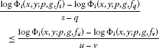
If and such that , then from (24) we have
If or , then opposite inequalities hold in (30).
Particularly, for and for , we have
and
respectively, where , , and are the same as defined in (29).
By taking in (26), () for , where are of the form

where , , and are the same as defined in (29).
If () are positive, then Theorem 2.4 applied to , and yields that there exists such that
Since the functions () are invertible for , we have
which together with the fact that () are continuous, symmetric and monotonous (by (25)) shows that are means.
Now, by the substitutions , , , (, ), where , from (31) we have
We define a new mean (for ) as follows:
These new means are also monotonous. More precisely, for such that , , , we have
We know that
equivalently
for such that , and , since () are monotonous in both parameters, so the claim follows. For , we obtain the required result by taking the limit .
Example 4.3
Consider the family of functions
defined by
We have , which shows that is convex for all . Since is the Laplace transform of a non-negative function (see [6, 7]), it is exponentially convex. It is easy to see that the function is also exponentially convex. Arguing as in Example 4.1, we have () are exponentially convex.
In this case, by taking in (26), () for , where are of the form

where , , and are the same as in (29). By using (25), () are monotonous in parameters s and q. By using Theorem 2.4, it can be seen that
satisfy and so () are means, where , , , is known as the logarithmic mean.
Example 4.4
Consider the family of functions
defined by
Here, , which shows that is convex for all . Since is the Laplace transform of a non-negative function (see [6, 7]), it is exponentially convex. It is easy to prove that the function is also exponentially convex. Arguing as in Example 4.1, we have () are exponentially convex.
In this case, by taking in (26), () for , where are of the form

where , , and are the same as in (29).
Remark 4.5
-
(i)
If () are positive, then applying Theorem 2.4 to in Examples 4.1, 4.3 and 4.4, we have
 (32)
(32)


and
() respectively, where , , , is known as the logarithmic mean. By using the same arguing as in Example 4.2, (32), (33) and (34) satisfy for , showing that () are means for . Also, from (25) it is clear that () for and are monotonous functions in parameters s and q.
-
(ii)
If we make the substitutions and in our means and (), then the results for the means and () given in [8] are recaptured. In this way, our results for means are the generalizations of the above mentioned means.
References
Franjić I, Khalid S, Pečarić J: On the refinements of the Jensen-Steffensen inequality. J. Inequal. Appl. 2011., 2011: Article ID 12
Pečarić J, Perić J: Improvements of the Giaccardi and the Petrović inequality and related Stolarsky type means. An. Univ. Craiova Ser. Mat. Inf. 2012, 39: 65–75.
Pečarić JE, Proschan F, Tong YL: Convex Functions, Partial Orderings and Statistical Applications. Academic Press, New York; 1992.
Butt SI, Krnić M, Pečarić J: Subadditivity, monotonicity and exponential convexity of the Petrović-type functionals. Abstr. Appl. Anal. 2012., 2012: Article ID 123913. doi:10.1155/2012/123913
Anwar M, Pečarić J: Means of the Cauchy Type. LAP Lambert Academic Publishing, Saarbrücken; 2009.
Jakšetić, J, Pečarić, J: Exponential convexity method. J. Convex Anal. (2013, in press)
Widder DV: The Laplace Transform. Princeton University Press, Princeton; 1941.
Khalid S, Pečarić J: On the refinements of the Hermite-Hadamard inequality. J. Inequal. Appl. 2012., 2012: Article ID 155
Acknowledgements
This research work was partially supported by the Higher Education Commission, Pakistan. The second author’s research was supported by the Croatian Ministry of Science, Education and Sports, under the Research Grant 117-1170889-0888.
Author information
Authors and Affiliations
Corresponding author
Additional information
Competing interests
The authors declare that they have no competing interests.
Authors’ contributions
Both authors worked jointly on the results and they read and approved the final manuscript.
Rights and permissions
Open Access This article is distributed under the terms of the Creative Commons Attribution 2.0 International License (https://creativecommons.org/licenses/by/2.0), which permits unrestricted use, distribution, and reproduction in any medium, provided the original work is properly cited.
About this article
Cite this article
Khalid, S., Pečarić, J. On the refinements of the integral Jensen-Steffensen inequality. J Inequal Appl 2013, 20 (2013). https://doi.org/10.1186/1029-242X-2013-20
Received:
Accepted:
Published:
DOI: https://doi.org/10.1186/1029-242X-2013-20