The collineations which act as addition and multiplication on points in a certain class of projective Klingenberg planes

Abstract

Let $P{K}_2(\mathbf{Q}(\epsilon ))$ be the projective Klingenberg plane coordinated by the dual quaternion ring $\mathbf{Q}(\epsilon )=\mathbf{Q}+\mathbf{Q}\epsilon =\{x+y\epsilon \mid x,y\in \mathbf{Q}\}$ where Q is any quaternion ring. In this paper, we determine the addition and multiplication of the points on the line $[0,1,0]$ of $P{K}_2(\mathbf{Q}(\epsilon ))$ as the image of some collineations of the plane $P{K}_2(\mathbf{Q}(\epsilon ))$. To do this, we give the collineations $S_a$ and $L_a$. Later we show that the addition and multiplication of the nonneighbor points on the line $[0,1,0]$ can be obtained as the images under that $S_a$ and $L_a$.

MSC:51C05, 51J10, 12E15.

1 Introduction and preliminaries

In the plane geometry, there are three important classes: affine planes, projective planes and hyperbolic planes. In recent years, studies on the generalization of these classes are becoming more popular. In this paper, we study on the projective Klingenberg planes, which are generalizations of the projective planes. Now we give some required concepts from [1–4] for understanding projective Klingenberg planes. A ring $\mathbf{R}:=(\mathbf{R},+,\cdot )$ is defined as a set R together with two binary operations + and ⋅, which we call addition and multiplication, such that the following axioms are satisfied:

R1: $(\mathbf{R},+)$ is an Abelian group;

R2: Multiplication is associative;

R3: Distributive laws holds.

A ring R with identity element is called local if the set I of its non-units forms an ideal.

A Projective Plane $\mathbf{\Pi }=(\mathcal{P},\mathcal{L},\in )$ is a system in which the elements of $\mathcal{P}$ are called points and the elements of ℒ are called lines together with an incidence relation ∈ between the points and lines such that

P1: If P and Q are distinct points, then there is a unique line passing through P and Q (denoted by $P\vee Q$ or PQ);

P2: If l and m are any lines, then there exist at least one point on both l and m;

P3: There exists four points such that no three of them are collinear.

In any projective plane, it is well known that there is a unique point on any distinct line pair and if l and m are distinct lines, the intersection point of these lines is denoted by $l\wedge m$ or lm.

A Projective Klingenberg plane (PK-Plane) is a system $(\mathcal{P},\mathcal{L},\in ,\sim )$ where $(\mathcal{P},\mathcal{L},\in )$ is an incidence structure and ∼ is an equivalence relation on $\mathcal{P}\cup \mathcal{L}$ (called neighboring) such that no point is neighbor to any line and the following axioms are satisfied:

PK1: If P and Q are non-neighbor points, then there is a unique line passing through P and Q;

PK2: If l and m are non-neighbor lines, then there is a unique point on both l and m;

PK3: There is a projective plane ${\mathbf{\Pi }}^{\ast }$ and an incidence structure epimorphism $\chi :\mathbf{\Pi }⟶{\mathbf{\Pi }}^{\ast }$ such that $P\sim Q⟺\chi (P)=\chi (Q)$ and $l\sim m⟺\chi (l)=\chi (m)$.

A point $P\in \mathcal{P}$ is called near a line $g\in \mathcal{L}$ (which is denoted by $P\sim g$) iff there exists a line $h\sim g$ such that $P\in h$.

An incidence structure automorphism preserving and reflecting the neighbor relation is called a collineation of Π.

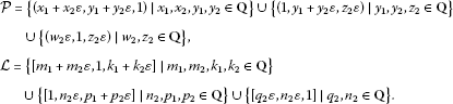
Let Π be a PK-plane with canonical image ${\mathbf{\Pi }}^{\ast }$. Choose a basis $(O,U,V,E)$ whose image $(\chi (O),\chi (U),\chi (V),\chi (E))$ in ${\mathbf{\Pi }}^{\ast }$ form a quadrangle. Let $g_{\mathrm{\infty }}:=UV$, $l:=OE$, $W:=l\wedge (UV)$, $\eta :=\{P\in l\mid P\sim O\}$ and $R:=\{P\in l\mid P\nsim W\}$. Let $0:=O$, $1:=E$. Then the points $P\in \mathcal{P}$ and the lines $g\in \mathcal{L}$ of Π get their coordinates as follows:

If $P\nsim g_{\mathrm{\infty }}$, let $P=(x,y,1)$ where $(x,x,1)=(PV)\wedge l$, $(y,y,1)=(PU)\wedge l$;

If $P\sim g_{\mathrm{\infty }}$, $P\nsim V$ let $P=(1,y,z)$ where $(1,z,1)=((PV\wedge UE)\vee O)\wedge EV$ and $(1,y,1)=OP\wedge EV$;

If $P\sim V$, let $P=(w,1,z)$ where $(1,1,z)=PU\wedge l$, and $(w,1,1)=OP\wedge EU$ (clearly $w,z\in \eta$);

If $g\nsim V$, then $g=[m,1,k]$ where $(1,m,1)=((g\wedge g_{\mathrm{\infty }})\vee O)\wedge EV$, $(0,k,1)=g\wedge OV$;

If $g\sim V$, $g\nsim g_{\mathrm{\infty }}$, then $g=[1,n,p]$ where $(n,1,1)=((g\wedge g_{\mathrm{\infty }})\vee O)\wedge EU$, $(p,0,1)=g\wedge OU$;

If $g\sim g_{\mathrm{\infty }}$, then $g=[q,n,1]$ where $(1,0,q)=g\wedge OU$, $(0,1,n)=g\wedge OV$ (then $q,n\in \eta$).

Then $O=(0,0,1)$, $U=(1,0,0)$, $V=(0,1,0)$, $E=(1,1,1)$, $OU=[0,1,0]$, $OV=[1,0,0]$, $UV=[0,0,1]$, $l=OE=[1,1,0]$ and a point $a\in \mathbf{R}$ has coordinates $(a,a,1)$. We note that $(a_1,a_2,a_3)\sim (b_1,b_2,b_3)$ if and only if $a_i-b_i\in \mathbf{I}$, for $i=1,2,3$, dually for lines.

Let R be a local ring and the set of the non-units is denoted by I. Now we recall a theorem and corollary which are constructed in [2] for Moufang-Klingenberg planes.

Theorem 1.1 The system $(\mathcal{P},\mathcal{L},\in ,\sim )$ is a PK-plane where

$$\begin{array}{r}\mathcal{P}=\{(x,y,1)\mid x,y\in \mathbf{R}\}\cup \{(1,y,z)\mid y\in \mathbf{R},z\in \mathbf{I}\}\cup \{(w,1,z)\mid w,z\in \mathbf{I}\},\\ \mathcal{L}=\{[m,1,k]\mid m,k\in \mathbf{R}\}\cup \{[1,n,p]\mid n\in \mathbf{I},p\in \mathbf{R}\}\cup \{[q,n,1]\mid q,n\in \mathbf{I}\},\\ (x,y,1)\in [m,1,k]\iff y=xm+k,\\ (x,y,1)\in [1,n,p]\iff x=yn+p,(x,y,1)\notin [q,n,1],\\ (1,y,z)\in [m,1,k]\iff y=m+zk,\\ (1,y,z)\in [q,n,1]\iff z=q+yn,(1,y,z)\notin [1,n,p],\\ (w,1,z)\in [1,n,p]\iff w=n+zp,\\ (w,1,z)\in [q,n,1]\iff z=wq+n,(w,1,z)\notin [m,1,k],\\ (x_1,x_2,x_3)\sim (y_1,y_2,y_3)\iff x_i-y_i\in \mathbf{I},\\ [a_1,a_2,a_3]\sim [b_1,b_2,b_3]\iff a_i-b_i\in \mathbf{I}.\end{array}$$

Corollary 1.2 If $t\in \mathbf{I}$, then $1-t$ is a unit and, therefore,

$$\begin{array}{r}(x,y,1)\nsim (1,y,z),(x,y,1)\nsim (w,1,z),(1,y,z)\nsim (w,1,z),\\ (w,1,z)\sim (u,1,t),(x,y,1)\sim (u,v,1)\iff (x-u\in \mathbf{I},y-v\in \mathbf{I}),\\ (1,y,z)\sim (1,v,t)\iff y-v\in \mathbf{I}.\end{array}$$

The PK-Plane given in Theorem 1.1 is denoted by $P{K}_2(\mathbf{R})$ and is called the PK-Plane coordinatized with (the local ring) R.

Finally we give the definition of dual quaternions, some theorems and a corollary from [5], which we use in the next section.

We consider any quaternion ring $\mathbf{Q}=\{x_0+x_{1}i+x_{2}j+x_{3}k\mid x_0,x_1,x_2,x_3\in \mathbf{F}\}$ over a field F (which is a division ring) and the set $\mathbf{Q}(\epsilon )=\mathbf{Q}+\mathbf{Q}\epsilon =\{a+b\epsilon \mid a,b\in \mathbf{Q}\}$ together with the following operations:

$$\begin{array}{r}(a+b\epsilon )+(c+d\epsilon )=(a+c)+(b+d)\epsilon ,\\ (a+b\epsilon )(c+d\epsilon )=ac+(ad+bc)\epsilon ,\end{array}$$

where ε represents any element not in Q.

The elements of $\mathbf{Q}(\epsilon )$ are called as dual quaternions. Obviously, the unity of $\mathbf{Q}(\epsilon )$ is 1.

Theorem 1.3 The non-unit elements of $\mathbf{Q}(\epsilon )$ are in the form bε, for $b\in \mathbf{Q}$ and if $a\ne 0$, $a,b\in Q$, then $a+b\epsilon$ is a unit and ${(a+b\epsilon )}^{-1}=a^{-1}-a^{-1}b{a}^{-1}\epsilon$.

Theorem 1.4 The set of non-units $\mathbf{I}=\mathbf{Q}\epsilon =\{b\epsilon \mid b\in \mathbf{Q}\}$ is an ideal of $\mathbf{Q}(\epsilon )$.

Corollary 1.5

• (1) $\mathbf{Q}(\epsilon )$ is a local ring (and it is called as the dual local ring on Q);

• (2) It is obvious from Theorem  1.1 that $P{K}_2(\mathbf{Q}(\epsilon ))=(\mathcal{P},\mathcal{L},\in ,\sim )$ is a PK-plane and

  

Theorem 1.6 Neighbor relation ∼ is an equivalence relation over $\mathcal{P}$ and ℒ in $P{K}_2(\mathbf{Q}(\epsilon ))$.

Theorem 1.7 In $P{K}_2(\mathbf{Q}(\epsilon ))$ the following properties are satisfied:

• (1) $(x_1+x_2\epsilon ,y_1+y_2\epsilon ,1)\in [m_1+m_2\epsilon ,1,k_1+k_2\epsilon ]⟺y_1=x_1{m}_1+k_1$, $y_2=x_2{m}_1+x_1{m}_2+k_2$;

• (2) $(x_1+x_2\epsilon ,y_1+y_2\epsilon ,1)\in [1,n_2\epsilon ,p_1+p_2\epsilon ]⟺x_1=p_1$, $x_2=y_1{n}_2+p_2$;

• (3) $(1,y_1+y_2\epsilon ,z_2\epsilon )\in [m_1+m_2\epsilon ,1,k_1+k_2\epsilon ]⟺y_1=m_1$, $y_2=m_2+z_2{k}_1$;

• (4) $(1,y_1+y_2\epsilon ,z_2\epsilon )\in [q_2\epsilon ,n_2\epsilon ,1]⟺z_2=q_2+y_1{n}_2$;

• (5) $(w_2\epsilon ,1,z_2\epsilon )\in [1,n_2\epsilon ,p_1+p_2\epsilon ]⟺w_2=n_2+z_2{p}_1$;

• (6) $(w_2\epsilon ,1,z_2\epsilon )\in [q_2\epsilon ,n_2\epsilon ,1]⟺z_2=n_2$;

• (7) $(a_1+a_2\epsilon ,b_1+b_2\epsilon ,1)\sim (c_1+c_2\epsilon ,d_1+d_2\epsilon ,1)⟺c_1=a_1\wedge d_1=b_1$;

• (8) $(1,a_1+a_2\epsilon ,b_2\epsilon )\sim (1,c_1+c_2\epsilon ,d_2\epsilon )⟺c_1=a_1$;

• (9) For every $a_2,b_2,c_2,d_2\in \mathbf{Q}$; $(a_2\epsilon ,1,b_2\epsilon )\sim (c_2\epsilon ,1,d_2\epsilon )$.

2 Two collineations of $P{K}_2(\mathbf{Q}(\epsilon ))$

In this section, we will define two transformations for the points and lines of $P{K}_2(\mathbf{Q}(\epsilon ))$ and also we will show that these transformations are collineations. Similar transformations can be found in [6].

Let $a=a_1+a_2\epsilon$ be an arbitrary element of $\mathbf{Q}(\epsilon )$. Then we define a transformation $S_a:P{K}_2(\mathbf{Q}(\epsilon ))⟶P{K}_2(\mathbf{Q}(\epsilon ))$ as:

$$\begin{array}{r}(x_1+x_2\epsilon ,y_1+y_2\epsilon ,1)⟶(x_1+a_1+(x_2+a_2)\epsilon ,y_1+y_2\epsilon ,1),\\ (1,y_1+y_2\epsilon ,z_2\epsilon )⟶(1,y_1+(y_2-z_2{a}_1{y}_1)\epsilon ,z_2\epsilon ),\\ (w_2\epsilon ,1,z_2\epsilon )⟶((w_2+z_2{a}_1)\epsilon ,1,z_2\epsilon ),\\ [m_1+m_2\epsilon ,1,k_1+k_2\epsilon ]⟶[m_1+m_2\epsilon ,1,k_1-a_1{m}_1+(k_2-a_1{m}_2-a_2{m}_1)\epsilon ],\\ [1,n_2\epsilon ,p_1+p_2\epsilon ]⟶[1,n_2\epsilon ,p_1+a_1+(p_2+a_2)\epsilon ],\\ [q_2\epsilon ,n_2\epsilon ,1]⟶[q_2\epsilon ,n_2\epsilon ,1].\end{array}$$

Similarly, we define a transformation $L_a:P{K}_2(\mathbf{Q}(\epsilon ))⟶P{K}_2(\mathbf{Q}(\epsilon ))$ where $a=a_1+a_2\epsilon \in \mathbf{Q}(\epsilon )$ and $a_1\ne 0$ as:

$$\begin{array}{r}(x_1+x_2\epsilon ,y_1+y_2\epsilon ,1)\\ ⟶(a_1{x}_1+(a_1{x}_2+a_2{x}_1)\epsilon ,a_1{y}_1{a}_1+(a_1{y}_1{a}_2+a_1{y}_2{a}_1+a_2{y}_1{a}_1)\epsilon ,1),\\ (1,y_1+y_2\epsilon ,z_2\epsilon )⟶(1,y_1{a}_1+(y_1{a}_2+y_2{a}_1)\epsilon ,\left(z_2{a}_1^{-1}\right)\epsilon ),\\ (w_2\epsilon ,1,z_2\epsilon )⟶(\left(a_1^{-1}{w}_2\right)\epsilon ,1,\left(a_1^{-1}{z}_2{a}_1^{-1}\right)\epsilon ),\\ [m_1+m_2\epsilon ,1,k_1+k_2\epsilon ]\\ ⟶[m_1{a}_1+(m_1{a}_2+m_2{a}_1)\epsilon ,1,a_1{k}_1{a}_1+(a_1{k}_1{a}_2+a_1{k}_2{a}_1+a_2{k}_1{a}_1)\epsilon ],\\ [1,n_2\epsilon ,p_1+p_2\epsilon ]⟶[1,\left(a_1^{-1}{n}_2\right)\epsilon ,a_1{p}_1+(a_1{p}_2+a_2{p}_1)\epsilon ],\\ [q_2\epsilon ,n_2\epsilon ,1]⟶[\left(q_2{a}_1^{-1}\right)\epsilon ,\left(a_1^{-1}{n}_2{a}_1^{-1}\right)\epsilon ,1].\end{array}$$

Now, we can give the following theorem.

Theorem 2.1 The transformations $S_a$ and $L_a$ defined above are collineations of $P{K}_2(\mathbf{Q}(\epsilon ))$.

Proof It must be shown that $S_a$ and $L_a$ are bijective and preserves the incidence and the neighbor relations.

It can be shown that $S_a$ and $L_a$ are one.to.one transformations. Also since;

$$\begin{array}{r}{S}_a(x_1-a_1+(x_2-a_2)\epsilon ,y_1+y_2\epsilon ,1)=(x_1+x_2\epsilon ,y_1+y_2\epsilon ,1),\\ S_a(1,y_1+(y_2+z_2{a}_1{y}_1)\epsilon ,z_2\epsilon )=(1,y_1+y_2\epsilon ,z_2\epsilon ),\\ S_a((w_2-z_2{a}_1)\epsilon ,1,z_2\epsilon )=(w_2\epsilon ,1,z_2\epsilon ),\\ S_a[m_1+m_2\epsilon ,1,k_1+a_1{m}_1+(k_2+a_1{m}_2+a_2{m}_1)\epsilon ]=[m_1+m_2\epsilon ,1,k_1+k_2\epsilon ],\\ S_a[1,n_2\epsilon ,p_1-a_1+(p_2-a_2)\epsilon ]=[1,n_2\epsilon ,p_1+p_2\epsilon ],\\ S_a[q_2\epsilon ,n_2\epsilon ,1]=[q_2\epsilon ,n_2\epsilon ,1]\end{array}$$

and

$$\begin{array}{r}{L}_a(a_1^{-1}{x}_1+\left(a_1^{-1}(x_2-a_2{a}_1^{-1}{x}_1)\right)\epsilon ,a_1^{-1}{y}_1{a}_1^{-1}+(a_1^{-1}((y_2-y_1{a}_1^{-1}{a}_2)a_1^{-1}-a_2{a}_1^{-1}{y}_1{a}_1^{-1})\epsilon ,1))\\ =(x_1+x_2\epsilon ,y_1+y_2\epsilon ,1),\\ L_a(1,y_1{a}_1^{-1}+\left((y_2-y_1{a}_1^{-1}{a}_2)a_1^{-1}\right)\epsilon ,(z_2{a}_1)\epsilon )=(1,y_1+y_2\epsilon ,z_2\epsilon ),\\ L_a((a_1{w}_2)\epsilon ,1,(a_1{z}_2{a}_1)\epsilon )=(w_2\epsilon ,1,z_2\epsilon ),\\ L_a[a_1^{-1}{m}_1+\left(a_1^{-1}(m_2-a_2{a}_1^{-1}{m}_1)\right)\epsilon ,1,a_1^{-1}{k}_1{a}_1^{-1}+\left(a_1^{-1}(k_2-k_1{a}_1^{-1}{a}_2-a_2{a}_1^{-1}{k}_1)a_1^{-1}\right)\epsilon ]\\ =[m_1+m_2\epsilon ,1,k_1+k_2\epsilon ],\\ L_a[1,(a_1{n}_2)\epsilon ,a_1^{-1}{p}_1+\left(a_1^{-1}(p_2-a_2{a}_1^{-1}{p}_1)\right)\epsilon ]=[1,n_2\epsilon ,p_1+p_2\epsilon ],\\ L_a[(q_2{a}_1)\epsilon ,(a_1{n}_2{a}_1)\epsilon ,1]=[q_2\epsilon ,n_2\epsilon ,1],\end{array}$$

we find that $S_a$ and $L_a$ are surjective and also since,

$$\begin{array}{r}{S}_a(x_1+x_2\epsilon ,y_1+y_2\epsilon ,1)\in S_a[m_1+m_2\epsilon ,1,k_1+k_2\epsilon ]\\ ⟺y_1+y_2\epsilon =(x_1+a_1+(x_2+a_2)\epsilon )(m_1+m_2\epsilon )+k_1-a_1{m}_1\\ \phantom{⟺y_1+y_2\epsilon =}+(k_2-a_1{m}_2-a_2{m}_1)\epsilon \\ ⟺y_1=x_1{m}_1+k_1\wedge y_2=x_1{m}_2+x_2{m}_1+k_2\\ ⟺(x_1+x_2\epsilon ,y_1+y_2\epsilon ,1)\in [m_1+m_2\epsilon ,1,k_1+k_2\epsilon ],\\ S_a(x_1+x_2\epsilon ,y_1+y_2\epsilon ,1)\in S_a[1,n_2\epsilon ,p_1+p_2\epsilon ]\\ ⟺x_1+a_1+(x_2+a_2)\epsilon =(y_1+y_2\epsilon )(n_2\epsilon )+p_1+a_1+(p_2+a_2)\epsilon \\ ⟺x_1=p_1\wedge x_2=y_1{n}_2+p_2\\ ⟺(x_1+x_2\epsilon ,y_1+y_2\epsilon ,1)\in [1,n_2\epsilon ,p_1+p_2\epsilon ],\\ S_a(1,y_1+y_2\epsilon ,z_2\epsilon )\in S_a[m_1+m_2\epsilon ,1,k_1+k_2\epsilon ]\\ ⟺y_1+(y_2-z_2{a}_1{y}_1)\epsilon =m_1+m_2\epsilon +(z_2\epsilon )(k_1-a_1{m}_1+(k_2-a_1{m}_2-a_2{m}_1)\epsilon )\\ ⟺y_1=m_1\wedge y_2=m_2+z_2{k}_1\\ ⟺(1,y_1+y_2\epsilon ,z_2\epsilon )\in [m_1+m_2\epsilon ,1,k_1+k_2\epsilon ],\\ S_a(1,y_1+y_2\epsilon ,z_2\epsilon )\in S_a[q_2\epsilon ,n_2\epsilon ,1]\\ ⟺z_2\epsilon =q_2\epsilon +(y_1+(y_2-z_2{a}_1{y}_1)\epsilon )(n_2\epsilon )\\ ⟺z_2\epsilon =q_2\epsilon +(y_1{n}_2)\epsilon \\ ⟺(1,y_1+y_2\epsilon ,z_2\epsilon )\in [q_2\epsilon ,n_2\epsilon ,1],\\ S_a(w_2\epsilon ,1,z_2\epsilon )\in S_a[1,n_2\epsilon ,p_1+p_2\epsilon ]\\ ⟺(w_2+z_2{a}_1)\epsilon =n_2\epsilon +(z_2\epsilon )(p_1+a_1+(p_2+a_2)\epsilon )\\ ⟺w_2=n_2+z_2{p}_1\\ ⟺(w_2\epsilon ,1,z_2\epsilon )\in [1,n_2\epsilon ,p_1+p_2\epsilon ],\\ S_a(w_2\epsilon ,1,z_2\epsilon )\in S_a[q_2\epsilon ,n_2\epsilon ,1]\\ ⟺z_2\epsilon =((w_2+z_2{a}_1)\epsilon )(q_2\epsilon )+n_2\epsilon \\ ⟺z_2\epsilon =n_2\epsilon \\ ⟺(w_2\epsilon ,1,z_2\epsilon )\in [q_2\epsilon ,n_2\epsilon ,1]\end{array}$$

and

$$\begin{array}{r}{L}_a(x_1+x_2\epsilon ,y_1+y_2\epsilon ,1)\in L_a[m_1+m_2\epsilon ,1,k_1+k_2\epsilon ]\\ ⟺y_1=x_1{m}_1+k_1\wedge y_2=x_1{m}_2+x_2{m}_1+k_2\\ ⟺(x_1+x_2\epsilon ,y_1+y_2\epsilon ,1)\in [m_1+m_2\epsilon ,1,k_1+k_2\epsilon ],\\ L_a(x_1+x_2\epsilon ,y_1+y_2\epsilon ,1)\in L_a[1,n_2\epsilon ,p_1+p_2\epsilon ]\\ ⟺x_1=p_1\wedge x_2=y_1{n}_2+p_2\\ ⟺(x_1+x_2\epsilon ,y_1+y_2\epsilon ,1)\in [1,n_2\epsilon ,p_1+p_2\epsilon ],\\ L_a(1,y_1+y_2\epsilon ,z_2\epsilon )\in L_a[m_1+m_2\epsilon ,1,k_1+k_2\epsilon ]\\ ⟺y_1=m_1\wedge y_2=m_2+z_2{k}_1\\ ⟺(1,y_1+y_2\epsilon ,z_2\epsilon )\in [m_1+m_2\epsilon ,1,k_1+k_2\epsilon ],\\ L_a(1,y_1+y_2\epsilon ,z_2\epsilon )\in L_a[q_2\epsilon ,n_2\epsilon ,1]\\ ⟺z_2=q_2+y_1{n}_2\\ ⟺(1,y_1+y_2\epsilon ,z_2\epsilon )\in [q_2\epsilon ,n_2\epsilon ,1],\\ L_a(w_2\epsilon ,1,z_2\epsilon )\in L_a[1,n_2\epsilon ,p_1+p_2\epsilon ]\\ ⟺w_2=n_2+z_2{p}_1\\ ⟺(w_2\epsilon ,1,z_2\epsilon )\in [1,n_2\epsilon ,p_1+p_2\epsilon ],\\ L_a(w_2\epsilon ,1,z_2\epsilon )\in L_a[q_2\epsilon ,n_2\epsilon ,1]\\ ⟺z_2\epsilon =n_2\epsilon \\ ⟺(w_2\epsilon ,1,z_2\epsilon )\in [q_2\epsilon ,n_2\epsilon ,1],\end{array}$$

we have that $S_a$ and $L_a$ preserves the incidence relation. Finally, since

$$\begin{array}{r}{S}_a(x_1+x_2\epsilon ,y_1+y_2\epsilon ,1)\sim S_a(u_1+u_2\epsilon ,v_1+v_2\epsilon ,1)\\ ⟺x_1-u_1=0\wedge y_1-v_1=0\\ ⟺(x_1+x_2\epsilon ,y_1+y_2\epsilon ,1)\sim (u_1+u_2\epsilon ,v_1+v_2\epsilon ,1),\\ S_a(1,y_1+y_2\epsilon ,z_2\epsilon )\sim S_a(1,v_1+v_2\epsilon ,t_2\epsilon )\\ ⟺y_1-v_1=0\\ ⟺(1,y_1+y_2\epsilon ,z_2\epsilon )\sim (1,v_1+v_2\epsilon ,t_2\epsilon ),\\ S_a(w_2\epsilon ,1,z_2\epsilon )\sim S_a(u_2\epsilon ,1,t_2\epsilon )\\ ⟺(w_2\epsilon ,1,z_2\epsilon )\sim (u_2\epsilon ,1,t_2\epsilon ),\\ S_a[m_1+m_2\epsilon ,1,k_1+k_2\epsilon ]\sim S_a[u_1+u_2\epsilon ,1,t_1+t_2\epsilon ]\\ ⟺m_1-u_1=0\wedge k_1-t_1=0\\ ⟺[m_1+m_2\epsilon ,1,k_1+k_2\epsilon ]\sim [u_1+u_2\epsilon ,1,t_1+t_2\epsilon ],\\ S_a[1,n_2\epsilon ,p_1+p_2\epsilon ]\sim S_a[1,v_2\epsilon ,t_1+t_2\epsilon ]\\ ⟺p_1-t_1=0\\ ⟺[1,n_2\epsilon ,p_1+p_2\epsilon ]\sim [1,v_2\epsilon ,t_1+t_2\epsilon ],\\ S_a[q_2\epsilon ,n_2\epsilon ,1]\sim S_a[u_2\epsilon ,v_2\epsilon ,1]\\ ⟺[q_2\epsilon ,n_2\epsilon ,1]\sim [u_2\epsilon ,v_2\epsilon ,1]\end{array}$$

and

$$\begin{array}{r}{L}_a(x_1+x_2\epsilon ,y_1+y_2\epsilon ,1)\sim L_a(u_1+u_2\epsilon ,v_1+v_2\epsilon ,1)\\ ⟺x_1-u_1=0\wedge y_1-v_1=0\\ ⟺(x_1+x_2\epsilon ,y_1+y_2\epsilon ,1)\sim (u_1+u_2\epsilon ,v_1+v_2\epsilon ,1),\\ L_a(1,y_1+y_2\epsilon ,z_2\epsilon )\sim L_a(1,v_1+v_2\epsilon ,t_2\epsilon )\\ ⟺y_1-v_1=0\\ ⟺(1,y_1+y_2\epsilon ,z_2\epsilon )\sim (1,v_1+v_2\epsilon ,t_2\epsilon ),\\ L_a(w_2\epsilon ,1,z_2\epsilon )\sim L_a(u_2\epsilon ,1,t_2\epsilon )\\ ⟺(w_2\epsilon ,1,z_2\epsilon )\sim (u_2\epsilon ,1,t_2\epsilon ),\\ L_a[m_1+m_2\epsilon ,1,k_1+k_2\epsilon ]\sim L_a[u_1+u_2\epsilon ,1,t_1+t_2\epsilon ]\\ ⟺m_1-u_1=0\wedge k_1-t_1=0\\ ⟺[m_1+m_2\epsilon ,1,k_1+k_2\epsilon ]\sim [u_1+u_2\epsilon ,1,t_1+t_2\epsilon ],\\ L_a[1,n_2\epsilon ,p_1+p_2\epsilon ]\sim L_a[1,v_2\epsilon ,t_1+t_2\epsilon ]\\ ⟺p_1-t_1=0\\ ⟺[1,n_2\epsilon ,p_1+p_2\epsilon ]\sim [1,v_2\epsilon ,t_1+t_2\epsilon ],\\ L_a[q_2\epsilon ,n_2\epsilon ,1]\sim L_a[u_2\epsilon ,v_2\epsilon ,1]\\ ⟺[q_2\epsilon ,n_2\epsilon ,1]\sim [u_2\epsilon ,v_2\epsilon ,1],\end{array}$$

we conclude that $S_a$ and $L_a$ preserves the neighbor relation. □

3 Addition and multiplication of points and their correspondences with collineations

In this section, we recall some definitions,theorems and results about geometric addition and multiplication of points on OU in $P{K}_2(\mathbf{Q}(\epsilon ))$ from [7] and also we will determine same relations between $S_a$, $L_a$ and geometric definitions of addition and multiplication of points on OU where $(O,U,V,E)$ is a base of $P{K}_2(\mathbf{Q}(\epsilon ))$.

Definition 3.1 Let A and B be non-neighbor points of $P{K}_2(\mathbf{Q}(\epsilon ))$ on the line OU. Then

• (1) $A+B$ is defined as the intersection point of the lines LV and OU where $L=KU\wedge BS$, $K=AV\wedge OS$, $S=(1,1,0)$;

• (2) $A\cdot B$ is defined as the intersection point of the lines VN and OU where $N=AS\wedge OM$, $M=BV\wedge 1S$, $S=(1,1,0)$, $1=(1,0,1)$.

Theorem 3.2 Let $A=(a_1+a_2\epsilon ,0,1)$ and $B=(b_1+b_2\epsilon ,0,1)$ be non-neighbor points on the line OU and $Z=(1,0,z_2\epsilon )$ be the point on the line OU (neighbor to U) then;

• (1) $A+B=((a_1+b_1)+(a_2+b_2)\epsilon ,0,1)$;

• (2) $A+Z=(1,0,z_2\epsilon )$;

• (3) $A\cdot B=(a_1{b}_1+(a_1{b}_2+a_2{b}_1)\epsilon ,0,1)$;

• (4) $A\cdot Z=(1,0,(z_2{a}_1^{-1})\epsilon )$ where $A\nsim O$;

• (5) $Z\cdot A=(1,0,(a_1^{-1}{z}_2)\epsilon )$ where $A\nsim O$.

Corollary 3.3 Following statements are valid where the points A, B, Z, O are defined as in Theorem  3.2 and Y is a point neighbor to $(0,0,1)$ (i.e. $Y\in \{(y_2\epsilon ,0,1)\mid x_2\in \mathbf{Q}\}$)

• (1) $A+B=B+A$ and $A+Z=Z+A$;

• (2) $A+O=A$ and $O+Z=Z$;

• (3) $A+Y\sim A$;

• (4) $A\cdot B\ne B\cdot A$;

• (5) $O\cdot A=A\cdot O=O$;

• (6) $1\cdot A=A=A\cdot 1$ and $1\cdot Z=Z=Z\cdot 1$;

• (7) $A\cdot Y\sim Y$ and $Y\cdot A\sim Y$.

Now we give a theorem which interprets the relation between the geometric addition and multiplication of points and the collineations $S_a$, $L_a$ which are given in last section.

Theorem 3.4 Following equalities are valid for the point $A=(a,0,1)$ and any point X on the line $OU=[0,1,0]$ where $a=a_1+a_2\epsilon \in \mathbf{Q}(\epsilon )$:

• (1) $S_a(X)=X+A$;

• (2) $L_a(X)=A\cdot X$ where $a_1\ne 0$.

Proof (1) If X is any non-neighbor point to U on the line OU, then there exist a $b_1+b_2\epsilon \in \mathbf{Q}(\epsilon )$ such that $X=(b_1+b_2\epsilon ,0,1)$. In this case,

$$S_a(X)=(b_1+a_1+(b_2+a_2)\epsilon ,0,1)=X+A.$$

If X is any point on the line OU neighbor to U, then there exist a $z_2\epsilon \in \mathbf{Q}(\epsilon )$ such that $X=(1,0,z_2\epsilon )$. In this case,

$$S_a(X)=(1,0+(0-z_2(a_{1}0))\epsilon ,z_2\epsilon )=(1,0,z_2\epsilon )=X+A.$$

• (2) If X is any non-neighbor point to U on the line OU then there exist a $b_1+b_2\epsilon \in \mathbf{Q}(\epsilon )$ such that $X=(b_1+b_2\epsilon ,0,1)$. In this case

  $$\begin{array}{rl}{L}_a(X)& =(a_1{b}_1+(a_1{b}_2+a_2{b}_1)\epsilon ,a_{1}0a_1+(a_{1}0a_2+a_{1}0a_1+a_{2}0a_1)\epsilon ,1)\\ =(a_1{b}_1+(a_1{b}_2+a_2{b}_1)\epsilon ,0,1)=A\cdot X.\end{array}$$

If X is any point on the line OU neighbor to U, then there exist a $z_2\epsilon \in \mathbf{Q}(\epsilon )$ such that $X=(1,0,z_2\epsilon )$. In this case,

$$L_a(X)=(1,0a_1+(0a_2+0a_1)\epsilon ,\left(z_2{a}_1^{-1}\right)\epsilon )=(1,0,\left(z_2{a}_1^{-1}\right)\epsilon )=A\cdot X.$$

Therefore, $S_a(X)=X+A$ and $L_a(X)=A\cdot X$ for any point X on $[0,1,0]$ where $A=(a,0,1)$. □

References

1. Akpinar A, Celik B, Ciftçi S: Cross-ratio and 6-figures in some Moufang-Klingenberg planes. Bull. Belg. Math. Soc. Simon Stevin 2008, 15: 49–64.
MathSciNet  Google Scholar
2. Baker CA, Lane ND, Lorimer JW: A coordinatization for Moufang-Klingenberg planes. Simon Stevin 1991, 65: 3–22.
3. Keppens D: Coordinazation of projective Klingenberg planes. Simon Stevin 1988, 62: 63–90.
4. Jacobson N 3. In Lectures in Abstract Algebra. 3rd edition. Springer, New York; 1980.
Google Scholar
5. Dayioglu A, Celik B: Projective Klingenberg planes constructed with dual local rings. AIP Conf. Proc. 2011, 1389: 308–311.
Article  Google Scholar
6. Celik B, Akpinar A, Ciftci S: 4-transitivity and 6-figures in some Moufang-Klingenberg planes. Monatshefte Math. 2007, 152: 283–294. 10.1007/s00605-007-0477-1
Article  MathSciNet  Google Scholar
7. Celik B, Erdogan FO: On the addition and multiplication of the points in a certain class of projective Klingenberg plane. International Congress in Honour of Professor Hari M. Srivastava at the Auditorium at the Campus of Uludag University 2012.
Download references
Acknowledgements
Dedicated to Professor Hari M Srivastava.
This work was supported by the Commission of Scientific Research Projects of Uludag University, Project number UAP(F)-2012/23.
Author information
Authors and Affiliations
Authors
Corresponding author
Correspondence to Basri Celik.
Additional information
Competing interests
The authors declare that they have no competing interests.
Authors’ contributions
Both authors have contributed equally to this paper. Both authors read and approved the final manuscript.
Rights and permissions
Open Access This article is distributed under the terms of the Creative Commons Attribution 2.0 International License (https://creativecommons.org/licenses/by/2.0), which permits unrestricted use, distribution, and reproduction in any medium, provided the original work is properly cited.
Reprints and permissions
About this article
Cite this article
Celik, B., Dayioglu, A. The collineations which act as addition and multiplication on points in a certain class of projective Klingenberg planes. J Inequal Appl 2013, 193 (2013). https://doi.org/10.1186/1029-242X-2013-193
Download citation
• Received:
• Accepted:
• Published:
• DOI: https://doi.org/10.1186/1029-242X-2013-193