The global solution of a diffusion equation with nonlinear gradient term

Abstract

Consider the viscosity solution to the initial boundary value problem of the diffusion equation

$$u_t=div\left({\left|\mathrm{\nabla }{u}^m\right|}^{p-2}\mathrm{\nabla }{u}^m\right)-u^{q_{1}m}{\left|\mathrm{\nabla }{u}^m\right|}^{p_1},$$

with $p>1$, $m>0$, $p_1\le 2$, $p>2p_1$, its initial value $u(x,0)=u_0(x)\in L^{q-1+\frac{1}{m}}(\mathrm{\Omega })$, $3>q>1$ and its boundary value $u(x,t)=0$, $(x,t)\in \partial \mathrm{\Omega }\times (0,\mathrm{\infty })$. If $p>1+\frac{1}{m}$, by considering the regularized problem and using Moser’s iteration technique, we get the locally uniformly bounded property of the solution and the locally bounded property of the $L^p$-norm of the gradient. By the compactness theorem, the existence of the viscosity solution of the equation is obtained provided that

$$\frac{mN{q}_1}{Nm(p-1)-N+mq}+\frac{p_1(m(p-1)+m-2)}{m(p-1)-1}<1.$$

If $2<p<1+\frac{1}{m}$, the existence of solution is obtained in a similar way, and the extinction of the solution is proved in this case.

MSC:35K55, 35K65, 35B40.

1 Introduction

The objective of the paper is to study the nonnegative weak solution of the following nonlinear parabolic equation:

(1.1)

(1.2)

(1.3)

where $\mathrm{\Omega }\subset {\mathbb{R}}^N$ is a bounded open domain, $p>1$, $m>0$, $p_1\le 2$, $p>2p_1$, $N\ge 1$, $0\le u_0(x)\in L^{q-1+\frac{1}{m}}(\mathrm{\Omega })$, $3>q>1$, and ∇ is the spatial gradient operator.

The equation of the form (1.1) was suggested as a mathematical model for a variety of problems in mechanics, physics and biology, which can be seen in [1–4]etc. It has been widely researched, whether it is linear (i.e., $m=1$, $p=2$, $p_1=0$, $m{q}_1=1$) or nonlinear, fast diffusion ($m(p-1)<1$) or slow diffusion ($m(p-1)>1$). For example, the existence of a nonnegative solution of (1.1)-(1.3) without the damping term $-u^{m{q}_1}{|\mathrm{\nabla }{u}^m|}^{p_1}$, defined in some weak sense, is well established (see [5, 6]). For other examples, Bertsh et al. [7] and Zhou et al. [8] discussed the existence and properties of viscosity solution for the equation

$$u_t=u\mathrm{△}u-\gamma {|\mathrm{\nabla }u|}^2,$$

(1.4)

where γ is a positive constant. Zhang et al. [9] discussed the existence and properties of the viscosity solution for the equation

$$u_t=\mathrm{△}u-a(x){|u|}^{q-1}{|\mathrm{\nabla }u|}^2,$$

(1.5)

where $a(x)$ is a known function.

The most important characteristic of equation (1.4) or (1.5) is in that, generally, the uniqueness of the solutions is not true; one can refer to [8–12]. Thus, for the equation of the type (1.1), we should mainly consider the existence of the viscosity solution (see Definition 1.2 below) and the related properties such as large time behaviors; one can refer to [13–16]etc. for some progress on this problem.

Now, we quote the following definition.

Definition 1.1 A nonnegative function $u(x,t)$ is called a weak solution of (1.1)-(1.3) if u satisfies

• (i)
  

  (1.6)
  

  (1.7)
  • (ii)
    $${\iint }_S[u{\phi }_t-{\left|\mathrm{\nabla }{u}^m\right|}^{p-2}\mathrm{\nabla }{u}^m\cdot \mathrm{\nabla }\phi -u^{m{q}_1}{\left|\mathrm{\nabla }{u}^m\right|}^{p_1}\phi ]dxdt=0,\mathrm{\forall }\phi \in C_0^1(S);$$

    (1.8)
  • (iii)
    $$\underset{t\to 0}{lim}{\int }_{\mathrm{\Omega }}|u(x,t)-u_0(x)|dx=0.$$

    (1.9)

  We will get the solution of (1.1)-(1.3) by considering the regularized problem

  $$u_t=div\left({({\left|\mathrm{\nabla }{u}^m\right|}^2+\frac{1}{k})}^{\frac{p-2}{2}}\mathrm{\nabla }{u}^m\right)-u^{m{q}_1}{\left|\mathrm{\nabla }{u}^m\right|}^{p_1},$$

  (1.10)

  with the initial value (1.2) and the homogeneous boundary value (1.3). The solutions of the regularized equation (1.10) are denoted by $u_k$.

  Definition 1.2 If $u_k$ is a solution of the initial boundary value problem of (1.10)-(1.2)-(1.3), ${lim}_{k\to \mathrm{\infty }}{u}_k=u$, a.e. in S, such that u is a weak solution of (1.1)-(1.3), then u is said to be a viscosity solution.

  The main aim of the paper is to show how the damping term $-u^{m{q}_1}|\mathrm{\nabla }{u}^{m{p}_1}|$ affects the equation, including how the damping term affects the existence of the solution and how the damping term affects the properties such as the extinction of the solution. By considering the solution $u_k$ of the regularized problem (1.10) and using Moser’s iteration technique, we get $u_k$’s local bounded properties and the local bounded properties of the $L^p$-norm of the gradient $\mathrm{\nabla }{u}_k$. By the compactness theorem, we get the existence of the viscosity solution of the diffusion equation itself. Apart from the general process of the proof such as in [3–5, 7, 9]etc., in which the main difficulty is how to prove that

  $${\left|\mathrm{\nabla }{u}_k^m\right|}^{\frac{p-2}{2}}\mathrm{\nabla }{u}_k^m\rightharpoonup (\ast )\chi ={\left|\mathrm{\nabla }{u}^m\right|}^{p-2}\mathrm{\nabla }{u}^m,\text{weakly star in }{L}_{\mathrm{loc}}^{\mathrm{\infty }}(0,\mathrm{\infty };L^{\frac{p}{p-1}}(\mathrm{\Omega })),$$

  in our paper, in addition to overcoming the above difficulty, we have to solve another difficulty lying in how to prove that

  $$-u_k^{m{q}_1}{\left|\mathrm{\nabla }{u}_k^m\right|}^{p_1}\rightharpoonup (\ast )\nu =-u^{m{q}_1}{\left|\mathrm{\nabla }{u}^m\right|}^{p_1},\text{weakly star in }{L}_{\mathrm{loc}}^{\mathrm{\infty }}(0,\mathrm{\infty };L^{\frac{p}{p_1}}(\mathrm{\Omega })).$$

  Also, we need to overcome the difficulty which comes from the damping term $-u^{m{q}_1}|\mathrm{\nabla }{u}^{m{p}_1}|$ when we prove the uniqueness of the viscosity solutions of (1.1)-(1.3).

  In order to get the desired results, some important relationships among the exponents $p_1$, $q_1$, q, p, m, N are imposed. We also need the following lemmas.

  Lemma 1.3 [17] (Gagliardo-Nirenberg)

  If $1\le l<N$, $1+\beta \le q$, $1\le r\le q\le (1+\beta )Nl/(N-l)$, suppose that $u^{1+\beta }\in W^{1,l}(\mathrm{\Omega })$, then

  $${\parallel u\parallel }_q\le c^{1/(1+\beta )}{\parallel u\parallel }_r^{1-\theta }{\parallel u^{1+\beta }\parallel }_{1,l}^{\theta /(1+\beta )},$$

  (1.11)

  where $\theta =(\beta +1)(r^{-1}-q^{-1})/(N^{-1}-l^{-1}+(\beta +1)r^{-1})$.

  Lemma 1.4 [18]

  Let $y(t)$ be a nonnegative function on $(0,T]$. If it satisfies

  $$y^{\prime }(t)+A{t}^{\lambda \theta -1}{y}^{1+\theta }(t)\le B{t}^{-k}y(t)+C{t}^{-\delta },0<t\le T,$$

  (1.12)

  where $A,\theta >0$, $\lambda \theta \ge 1$, $B,C\ge 0$, $k\le 1$, then

  $$y(t)\le A^{-\frac{1}{\theta }}{(2\lambda +2B{T}^{1-k})}^{\frac{1}{\theta }}{t}^{-\lambda }+2C{(\lambda +B{T}^{1-k})}^{-1}{t}^{1-\delta },0<t\le T.$$

  (1.13)

  We will prove the following theorems. As usual, the constants c in what follows may be different from one to another.

  Theorem 1.5 If $0\le u_0(x)$ and

  

  (1.14)
  

  (1.15)
  

  (1.16)
  

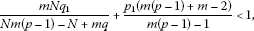  (1.17)

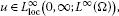
  then (1.1)-(1.3) has a weak viscosity solution which satisfies

  

  (1.18)

  and

  $${\parallel u^m(t)\parallel }_{\mathrm{\infty }}\le c(1+t^{-\lambda }){(1+t)}^{-1/(p-1-\frac{1}{m})},t>0,$$

  (1.19)

  where $\lambda =N{(pq+(p-1-\frac{1}{m})N)}^{-1}$. Moreover, if $p>2$, then

  $${\parallel \mathrm{\nabla }{u}^m\parallel }_p\le c(1+t^{-\mu }){(1+t)}^{-\sigma },t>0,$$

  (1.20)

  where $\mu =1+\frac{m-1}{m(p-1)-1}$, $\sigma =\frac{p(m(2q_1+1)-1)+m{p}_1}{(m(p-1)-1)(p-p_1)}$.

  The condition (1.17) is only used to prove (1.9); if $p_1=0=q_1$, this is a natural condition. We conjecture that this condition can be weakened.

  Theorem 1.6 Let u be a weak solution of (1.1)-(1.3). If $p>1+\frac{1}{m}$, $p_1+q_1>p-1$, then

  $$suppu(\cdot ,s)\subset suppu(\cdot ,t)$$

  (1.21)

  for all s, t with $0<s<t$.

  Theorem 1.7 If $2<p<1+\frac{1}{m}<p+q$,

  $$0\le u_0\in L^{q-1+\frac{1}{m}}(\mathrm{\Omega }),3>q>1,$$

  (1.22)

  then (1.1)-(1.3) has a weak solution which satisfies (1.18), and there exists a positive $T>0$ such that

  $$u(x,t)\equiv 0,\mathrm{\forall }(x,t)\in (x,t)\in \overline{\mathrm{\Omega }}\times (T,\mathrm{\infty }).$$

  (1.23)

  If the damping term disappears in (1.1), say, if (1.1) without $-u^{m{q}_1}|\mathrm{\nabla }{u}^{m{p}_1}|$ by [19], then we know that the extinction of the solution as Theorem 1.7 is true. For other related works on equation (1.1), one can refer to the references [20–31]etc. We use some ideas in [19] and [30].

2 The $L^{\mathrm{\infty }}$ estimate of the solution

Consider the regularized problem

(2.1)

(2.2)

(2.3)

where $0\le u_{0k}(x)$ is a suitably smooth function such that

$$u_0(x)\in L^{\mathrm{\infty }}(\mathrm{\Omega }),\underset{k\to \mathrm{\infty }}{lim}{\parallel u_{0k}\parallel }_{q-1+\frac{1}{m}}={\parallel u_0\parallel }_{q-1+\frac{1}{m}}.$$

Clearly,

$$|-u^{m{q}_1}{\left|\mathrm{\nabla }{u}^m\right|}^{p_1}|=m^{p_1}\left|u^{m{q}_1+p_1(m-1)}{|\mathrm{\nabla }u|}^{p_1}\right|,$$

if let

$$b(x,t,z,p)=-m^{p_1}\left|z^{m{q}_1+p_1(m-1)}{|p|}^{p_1}\right|.$$

Then, if $|z|\le M$, since $p_1\le 2$,

$$|b|\le c{|p|}^2,$$

by Chapter 8 of [32], viewing (2.1) as a divergent form of a quasilinear parabolic equation, we know that (2.1)-(2.3) has a unique nonnegative classical solution $u_k$. In what follows, in the proof of the related lemmas, we only denote $u_k$ as u for simplicity.

Lemma 2.1 If $p>1+\frac{1}{m}$, $u_k$ is the solution of (2.1)-(2.3), then $u_k^m\in L_{\mathrm{loc}}^{\mathrm{\infty }}(0,\mathrm{\infty };L^{q-1+\frac{1}{m}}(\mathrm{\Omega }))$ and

$${\parallel u_k^m\parallel }_{q-1+\frac{1}{m}}\le c{(1+t)}^{-\frac{1}{p-1-\frac{1}{m}}},t\ge 0,$$

(2.4)

where $3>q>1$.

Proof Let $A_n=(q-2)n^{3-q}$, $B_n=(3-q)n^{2-q}$ and

$$f_n(s)=\{\begin{array}{cc}{s}^{q-1}\hfill & \text{if }s\ge \frac{1}{n},\hfill \\ A_n{s}^2+B_{n}s\hfill & \text{if }0\le s<\frac{1}{n}.\hfill \end{array}$$

The condition $3>q>1$ assures that $f(u^m)$ defined above is nonnegative. If we multiply (2.1) by $f_n(u^m)$ and integral on Ω, then we have

(2.5)

(2.6)

From the above calculation, we have

$${\int }_{\mathrm{\Omega }}{f}_n\left(u^m\right)u_{t}dx+{\int }_{\mathrm{\Omega }}{\left|\mathrm{\nabla }{\int }_0^{u^m}{(f_n^{\prime }(s))}^{\frac{1}{p}}ds\right|}^{p}dx\le 0.$$

By the Poincare inequality, we have

$${\int }_{\mathrm{\Omega }}{f}_n\left(u^m\right)u_{t}dx+c{\int }_{\mathrm{\Omega }}{\left|{\int }_0^{u^m}{(f_n^{\prime }(s))}^{\frac{1}{p}}ds\right|}^{p}dx\le 0.$$

(2.7)

Let $n\to \mathrm{\infty }$ in (2.7). We can deduce that

$$\frac{d}{dt}{\int }_{\mathrm{\Omega }}{u}^{m(q-1)+1}dx+c{\int }_{\mathrm{\Omega }}{u}^{m[q-1+\frac{1}{m}+p-1-\frac{1}{m}]}dx\le 0.$$

(2.8)

By the Jessen inequality, from (2.8) we get

$$\frac{d}{dt}{\parallel u^m\parallel }_{q-1+\frac{1}{m}}^{q-1+\frac{1}{m}}+c{\parallel u^m\parallel }_{q-1+\frac{1}{m}}^{q-1+\frac{1}{m}+p-1-\frac{1}{m}}\le 0,$$

then

$${\parallel u^m\parallel }_{q+1-\frac{1}{m}}\le c{(1+t)}^{-\frac{1}{p-1-\frac{1}{m}}}.$$

We get the desired result. □

Lemma 2.2 If $p>1+\frac{1}{m}$, $u_k$ is the solution of (2.1)-(2.3), then

(2.9)

(2.10)

where $\lambda =\frac{N}{(p-1-\frac{1}{m})N+q}$.

Proof Multiply (2.1) by $u^{m(l-1)}$ and integral on Ω, then

$$\begin{array}{rcl}{\int }_{\mathrm{\Omega }}{u}^{m(l-1)}{u}_{t}dx& =& {\int }_{\mathrm{\Omega }}div\left({(\left|\mathrm{\nabla }{u}^m\right|+\frac{1}{k})}^{\frac{p-2}{2}}\mathrm{\nabla }{u}^m\right)u^{m(l-1)}dx\\ -{\int }_{\mathrm{\Omega }}{u}^{m{q}_1}{\left|\mathrm{\nabla }{u}^m\right|}^{p_1}{u}^{m(l-1)}dx\\ =& -(l-1){\int }_{\mathrm{\Omega }}{(\left|\mathrm{\nabla }{u}^m\right|+\frac{1}{k})}^{\frac{p-2}{2}}{\left|\mathrm{\nabla }{u}^m\right|}^2{u}^{m(l-2)}dx\\ -{\int }_{\mathrm{\Omega }}{u}^{m{q}_1}{\left|\mathrm{\nabla }{u}^m\right|}^{p_1}{u}^{m(l-1)}dx\\ \le & -(l-1){\int }_{\mathrm{\Omega }}{(\left|\mathrm{\nabla }{u}^m\right|+\frac{1}{k})}^{\frac{p-2}{2}}{\left|\mathrm{\nabla }{u}^m\right|}^2{u}^{m(l-2)}dx,\end{array}$$

which deduces that

$$\frac{d}{dt}{\parallel u^m\parallel }_{l-1+\frac{1}{m}}^{l-1+\frac{1}{m}}+c{(l-1+\frac{1}{m})}^{2-p}{\int }_{\mathrm{\Omega }}{\left|\mathrm{\nabla }{u}^{m\frac{p+l-1+\frac{1}{m}-1-\frac{1}{m}}{p}}\right|}^{p}dx\le 0.$$

Set $L=l-1+\frac{1}{m}$. Then

$$\frac{d}{dt}{\parallel u^m\parallel }_L^L+c{L}^{2-p}{\int }_{\mathrm{\Omega }}{\left|\mathrm{\nabla }{u}^{m\frac{L+p-1-\frac{1}{m}}{p}}\right|}^{p}dx\le 0,$$

(2.11)

where c is a constant independent of l.

Now, if we choose $L_1=q-1-\frac{1}{m}$, $L_n=r{L}_{n-1}-(p-1-\frac{1}{m})$, ${\theta }_n=rN(1-L_{n-1}{L}_n^{-1}){(p+N(r-1))}^{-1}$, ${\mu }_n=(L_n+p-1-\frac{1}{m}){\theta }_n^{-1}-L_n$, $r>1+(p-1-\frac{1}{m})q^{-1}$, $n=2,3,\dots$ , by Lemma 1.3, we have

$${\parallel u^m\parallel }_{L_n}\le c^{p/(L_n+p-1-\frac{1}{m})}{\parallel u^m\parallel }_{L_{n-1}}^{1-{\theta }_n}{\parallel \mathrm{\nabla }{u}^{m(L_n+p-1-\frac{1}{m})/p}\parallel }_p^{p{\theta }_n/(p-1-\frac{1}{m}+L_n)}.$$

(2.12)

If we choose $L=L_n$ in (2.11), by (2.12) we have

$$\frac{d}{dt}{\parallel u^m\parallel }_{L_n}^{L_n}+c^{-p/{\theta }_n}{L}_n^{2-p}{\parallel u^m\parallel }_{L_n}^{L_n+{\mu }_n}{\parallel u^m\parallel }_{L_{n-1}}^{p-1-\frac{1}{m}-{\mu }_n}\le 0,0<t\le 1.$$

(2.13)

We will prove that there exist two bounded sequences $\{{\xi }_n\}$, $\{{\lambda }_n\}$ such that

$${\parallel u^m\parallel }_{L_n}\le {\xi }_n{t}^{-{\lambda }_n},0<t\le 1.$$

(2.14)

If $n=1$, by Lemma 2.1, ${\lambda }_1=0$, ${\xi }_1={sup}_{t\ge 0}{\parallel u^m(t)\parallel }_{q-1-\frac{1}{m}}$ makes (2.14) sure. If (2.14) is true for $n-1$, then from (2.13),

$$\frac{d}{dt}{\parallel u^m\parallel }_{L_n}^{L_n}+c^{-p/{\theta }_n}{L}_n^{2-p}{\parallel u^m\parallel }_{L_n}^{L_n+{\mu }_n}{\xi }_{n-1}^{p-1-\frac{1}{m}-{\mu }_n}{t}^{-(p-1-\frac{1}{m}-{\mu }_n){\lambda }_{n-1}}\le 0,0<t\le 1.$$

(2.15)

We can choose

$${\lambda }_n=({\lambda }_{n-1}({\mu }_n-p+1+\frac{1}{m})+1){\mu }_n^{-1},{\xi }_n={\xi }_{n-1}{\left(c^{p/{\theta }_n}{L}_n^{p-1}{\lambda }_n\right)}^{1/{\mu }_n},n=2,3,\dots ,$$

by Lemma 1.4 and (2.15), (2.14) is true.

Moreover, by Lemma 1.4, as $n\to \mathrm{\infty }$, ${\lambda }_n\to \lambda =\frac{N}{(p-1-\frac{1}{m})N+q}$. It is easy to see that $\{{\xi }_n\}$ is bounded. Thus (2.9) is true.

To prove (2.10), we set $\tau =log(1+t)$, $t\ge 1$, $w(\tau )={(1+t)}^{\frac{1}{p-1-\frac{1}{m}}}{u}^m(t)$. By (2.11), we have

$$\frac{d}{d\tau }{\parallel w(\tau )\parallel }_L^L+c{L}^{2-p}{\parallel \mathrm{\nabla }{w}^{\frac{L+p-1-\frac{1}{m}}{p}}\parallel }_p^p\le \frac{L}{p-1-\frac{1}{m}}{\parallel w(\tau )\parallel }_L^L,\tau \ge log2.$$

(2.16)

By Lemma 3.1 in [31], we can get (2.10); we omit details here. □

3 The $L^{\mathrm{\infty }}$ estimation of the gradient

Lemma 3.1 If $p>max\{2,1+\frac{1}{m}\}$, $u_k$ is the solution of (2.1)-(2.3), then

(3.1)

(3.2)

Proof If we multiply (3.1) by $u_t^m$ and integral on Ω, then

(3.3)

(3.4)

(3.5)

By (3.3)-(3.5), we have

$${\int }_{\mathrm{\Omega }}{u}^{m-1}{(u_t)}^{2}dx+\frac{1}{m}\frac{d}{dt}{\mathrm{\Gamma }}_k\left({\left|\mathrm{\nabla }{u}^m\right|}^2\right)\le c{\int }_{\mathrm{\Omega }}{\left|u^m\right|}^{2p_1+\frac{m-1}{m}}{\left|\mathrm{\nabla }{u}^m\right|}^{2p_1}dx.$$

(3.6)

If we multiply (3.1) by $u^m$ and integral on Ω, then

$$\begin{array}{rcl}\frac{1}{m+1}{\int }_{\mathrm{\Omega }}\frac{d}{dt}{u}^{m+1}dx& =& {\int }_{\mathrm{\Omega }}div\left({({\left|\mathrm{\nabla }{u}^m\right|}^2+\frac{1}{k})}^{\frac{p-2}{2}}\mathrm{\nabla }{u}^m\right)u^{m}dx-{\int }_{\mathrm{\Omega }}{u}^{m{q}_1}{\left|\mathrm{\nabla }{u}^m\right|}^{p_1}{u}^{m}dx\\ =& -{\int }_{\mathrm{\Omega }}{({\left|\mathrm{\nabla }{u}^m\right|}^2+\frac{1}{k})}^{\frac{p-2}{2}}{\left|\mathrm{\nabla }{u}^m\right|}^{2}dx-{\int }_{\mathrm{\Omega }}{u}^{m{q}_1}{\left|\mathrm{\nabla }{u}^m\right|}^{p_1}{u}^{m}dx\end{array}$$

and

$$\begin{array}{rcl}{\mathrm{\Gamma }}_k\left({\left|\mathrm{\nabla }{u}^m\right|}^2\right)& \le & {\int }_{\mathrm{\Omega }}{({\left|\mathrm{\nabla }{u}^m\right|}^2+\frac{1}{k})}^{\frac{p-2}{2}}{\left|\mathrm{\nabla }{u}^m\right|}^{2}dx\\ =& -\frac{1}{m+1}{\int }_{\mathrm{\Omega }}\frac{d}{dt}{u}^{m+1}dx-{\int }_{\mathrm{\Omega }}{u}^{m{q}_1}{\left|\mathrm{\nabla }{u}^m\right|}^{p_1}{u}^{m}dx\\ \le & \frac{1}{m+1}{\parallel u^{\frac{m+1}{2}}\parallel }_2{\parallel u^{\frac{m-1}{2}}{u}_t\parallel }_2.\end{array}$$

So,

(3.7)

Setting $2\gamma =2q_1+1-\frac{1}{m}$, for $\mathrm{\forall }a\in [0,2\gamma ]$, if we notice that $p>2p_1$, we have

$${\int }_{\mathrm{\Omega }}{\left|u^m\right|}^{2a}{\left|\mathrm{\nabla }{u}^m\right|}^{2p_1}dx\le {\parallel u^m(t)\parallel }_{\mathrm{\infty }}^a{\left({\int }_{\mathrm{\Omega }}{\left|u^m\right|}^{\frac{(2\gamma -a)p}{p-2p_1}}dx\right)}^{\frac{p-2p_1}{p}}{\parallel \mathrm{\nabla }{u}^m\parallel }_p^{2p_1}.$$

(3.8)

If $2\gamma \ge (p-2p_1)(N+1)/N$, let $a={(2\gamma -(p-2p_1)(1+\frac{q}{N}))}^{+}$. By Lemma 1.3,

$${\left({\int }_{\mathrm{\Omega }}{\left|u^m\right|}^{\frac{(2\gamma -a)p}{p-2p_1}}dx\right)}^{\frac{p-2p_1}{p}}\le c{\parallel u^m(t)\parallel }_s^{(2\gamma -a)(1-\theta )}{\parallel \mathrm{\nabla }{u}^m\parallel }_p^{p-2p_1},$$

(3.9)

where $\theta =(s^{-1}-(1-\frac{2p_1}{p}){(2\gamma -a)}^{-1})/(N^{-1}-p^{-1}+s^{-1})$, and $s=(2\gamma -p+2p_1-a)N/(p-2p_1)$ when $2\gamma \ge (p-2p_1)(1+q/N)$, $s=q$, when $(p-2p_1)(1+N^{-1})\le 2\gamma \le (p-2p_1)(1+q/N)$. By Lemma 2.1 and Lemma 2.2, from (3.8), we have

$${\int }_{\mathrm{\Omega }}{\left|u^m\right|}^{2a}{\left|\mathrm{\nabla }{u}^m\right|}^{2p_1}dx\le c{t}^{-\lambda a}{\parallel \mathrm{\nabla }{u}^m\parallel }_p^p\le c{t}^{-\lambda a}{\mathrm{\Gamma }}_k\left({\left|\mathrm{\nabla }{u}^m\right|}^2\right),0<t\le 1.$$

(3.10)

At the same time, if we choose $q=2$ in Lemma 2.1, we have

$${\parallel u^m\parallel }_{1+\frac{1}{m}}={\left({\int }_{\mathrm{\Omega }}{u}^{m+1}dx\right)}^{\frac{m}{m+1}}\le c{t}^{-{(p-1-\frac{m}{m+1})}^{-1}}$$

and

$${\parallel u^{\frac{m+1}{2}}\parallel }_2^2={\int }_{\mathrm{\Omega }}{u}^{m+1}dx\le c{t}^{-\frac{m+1}{m(p-1)-1}}.$$

(3.11)

By (3.7), we have

$${\mathrm{\Gamma }}_k^{\prime }(t)+c{t}^{\frac{m+1}{m(p-1)-1}}{\mathrm{\Gamma }}_k^2(t)\le c{t}^{-\lambda a}{\mathrm{\Gamma }}_k(t),0<t\le 1.$$

(3.12)

If $2\gamma <(p-2p_1)(N+1)/N$ and $p-2p_1\le 2a\le 2\gamma$, then

$$\begin{array}{rcl}{\int }_{\mathrm{\Omega }}{\left|u^m\right|}^{2a}{\left|\mathrm{\nabla }{u}^m\right|}^{2p_1}dx& \le & c{\parallel \mathrm{\nabla }{u}^m\parallel }_1^{2a(1-\theta )}{\parallel \mathrm{\nabla }{u}^m\parallel }_p^{2a\theta +2p_1}\le c{\parallel \mathrm{\nabla }{u}^m\parallel }_p^p\le c{\mathrm{\Gamma }}_k\left({\left|\mathrm{\nabla }{u}^m\right|}^2\right),\\ 0<t\le 1.\end{array}$$

(3.13)

If $2\gamma <(p-2p_1)(N+1)/N$ and $p-2\ge 2a\ge 0$, then

$$\begin{array}{rcl}{\int }_{\mathrm{\Omega }}{\left|u^m\right|}^{2a}{\left|\mathrm{\nabla }{u}^m\right|}^{2}dx& \le & c(1+{\parallel \mathrm{\nabla }{u}^m\parallel }_p^p)\le c(1+{\mathrm{\Gamma }}_k\left({\left|\mathrm{\nabla }{u}^m\right|}^2\right)),\\ 0<t\le 1.\end{array}$$

(3.14)

The inequalities (3.13) and (3.14) mean that the inequality (3.12) is still true when $2\gamma <(p-2p_1)(N+1)/N$. Using Lemma 1.4, we get

$${\mathrm{\Gamma }}_k(t)\le c{t}^{-(1+\frac{m-1}{m(p-1)-1})},0<t\le 1,$$

which means (3.1) is true. Now, we will prove (3.2). For $t\ge 1$, by (2.10) we obtain

(3.15)

(3.16)

(3.17)

By (3.7), using (3.15)-(3.17) yields

$${\mathrm{\Gamma }}_k^{\prime }(t)+c{(1+t)}^{-{(p-1-\frac{1}{m})}^{-1}}{\mathrm{\Gamma }}_k^2(t)\le c{(1+t)}^{2\gamma /(p-1-\frac{1}{m})}{({\mathrm{\Gamma }}_k(t))}^{\frac{2p_1}{p}},$$

and using the Young inequality gives

$$\begin{array}{rcl}{\mathrm{\Gamma }}_k^{\prime }(t)+c{(1+t)}^{-{(p-1-\frac{1}{m})}^{-1}}{\mathrm{\Gamma }}_k^2(t)& \le & c{(1+t)}^{\frac{-m(2\gamma p+p_1)}{(m(p-1)-1)(p-p_1)}}\\ =& c{(1+t)}^{-\frac{p(m(2q_1+1)-1)+m{p}_1}{(m(p-1)-1)(p-p_1)}},\end{array}$$

which means (3.2) is true. □

Lemma 3.2 If $p>1+\frac{1}{m}$, $u_k$ is the solution of (2.1)-(2.3), then

$${\int }_t^T{\int }_{\mathrm{\Omega }}{u}_k^{m-1}{(u_{kt})}^{2}dxds\le c{t}^{-(1+\frac{m-1}{m(p-1)-1})}+c{t}^{-(\lambda \gamma +\frac{m-1}{m(p-1)-1})},0<t\le T.$$

(3.18)

Proof From (2.9), (3.1) and (3.7), (3.10), we have

$$\begin{array}{rcl}{\int }_t^T{\int }_{\mathrm{\Omega }}{u}^{m-1}{(u_t)}^{2}dxds& \le & {\mathrm{\Gamma }}_k(t)+c{\int }_t^T{\int }_{\mathrm{\Omega }}{\left|u^m\right|}^{2q_1+\frac{m-1}{m}}{\left|\mathrm{\nabla }{u}^m\right|}^{2p_1}dxds\\ \le & {\mathrm{\Gamma }}_k(t)+c{\int }_t^T{s}^{-\frac{\lambda }{2}(2q_1+\frac{m-1}{m})}{\mathrm{\Gamma }}_k(s)ds\\ \le & c{t}^{-(1+\frac{m-1}{m(p-1)-1})}+c{t}^{-(\lambda \gamma +\frac{m-1}{m(p-1)-1})}.\end{array}$$

(3.19)

 □

4 The proof of Theorem 1.5

The proof of Theorem 1.5 From Lemma 2.1, Lemma 2.2, Lemma 3.1 and Lemma 3.2, using the compactness theory (cf. [17]), there is a sequence (still denoted as$\{u_k\}$) of $\{u_k\}$ such that when $k\to \mathrm{\infty }$, we have

(4.1)

(4.2)

(4.3)

(4.4)

where $\chi =\{{\chi }_i:1\le i\le N\}$ and every ${\chi }_i$ is a function in $L_{\mathrm{loc}}^{\mathrm{\infty }}(0,T;L^{\frac{p}{p-1}}(\mathrm{\Omega }))$, $\nu \in L_{\mathrm{loc}}^{\mathrm{\infty }}(0,\mathrm{\infty };L^{\frac{p}{p_1}}(\mathrm{\Omega }))$. (4.1) and (4.2) are clearly true. In what follows, we only need to prove that

$$\chi ={\left|\mathrm{\nabla }{u}^m\right|}^{p-2}\mathrm{\nabla }{u}^m\text{in }{L}_{\mathrm{loc}}^{\mathrm{\infty }}(0,\mathrm{\infty };L^{\frac{p}{p-1}}(\mathrm{\Omega }))$$

(4.5)

and

$$\nu =u^{m{q}_1}{\left|\mathrm{\nabla }{u}^m\right|}^{p_1}\text{in }{L}_{\mathrm{loc}}^{\mathrm{\infty }}(0,\mathrm{\infty };L^{\frac{p}{p_1}}(\mathrm{\Omega })).$$

(4.6)

It is easy to know that

$${\iint }_S(u{\phi }_t-\chi \cdot \mathrm{\nabla }\phi -\nu \phi )dxdt=0,\mathrm{\forall }\phi \in C_0^{\mathrm{\infty }}(S).$$

(4.7)

So, if we can prove that

(4.8)

(4.9)

then (4.5),(4.6) and (1.8) are true.

First, for any $\psi \in C_0^{\mathrm{\infty }}(S)$, $0\le \psi \le 1$, $v^m\in L_{\mathrm{loc}}^p(0,T;W_0^{1,p}(\mathrm{\Omega }))$, we have

$${\iint }_S\psi ({\left|\mathrm{\nabla }{u}_k^m\right|}^{p-2}\mathrm{\nabla }{u}_k^m-{\left|\mathrm{\nabla }{v}^m\right|}^{p-2}\mathrm{\nabla }{v}^m)\cdot \mathrm{\nabla }(u_k^m-v^m)dxdt\ge 0.$$

(4.10)

If we multiply by $u_k^m\psi$ the two sides of (2.1), then we have

(4.11)

Noticing that when $1<p<2$, we have

and when $p\ge 2$, we get

$${({\left|\mathrm{\nabla }{u}_k^m\right|}^2+\frac{1}{k})}^{\frac{p-2}{2}}{\left|\mathrm{\nabla }{u}_k^m\right|}^2\ge {\left|\mathrm{\nabla }{u}_k^m\right|}^p,{({\left|\mathrm{\nabla }{u}_k^m\right|}^2+\frac{1}{k})}^{\frac{p-2}{2}}\left|\mathrm{\nabla }{u}_k^m\right|\le ({\left|\mathrm{\nabla }{u}_k^m\right|}^{p-1}+1).$$

By (4.10), (4.11), we have

(4.12)

Since

$${({\left|\mathrm{\nabla }{u}_k^m\right|}^2+\frac{1}{k})}^{\frac{p-2}{2}}\mathrm{\nabla }{u}_k^m={\left|\mathrm{\nabla }{u}_k^m\right|}^{p-2}\mathrm{\nabla }{u}_k^m+\frac{p-2}{2k}{\int }_0^1{({\left|\mathrm{\nabla }{u}_k^m\right|}^2+\frac{s}{k})}^{\frac{p-4}{2}}ds\mathrm{\nabla }{u}_k^m$$

and

$$\underset{k\to \mathrm{\infty }}{lim}\frac{p-2}{2k}{\iint }_S{\int }_0^1{({\left|\mathrm{\nabla }{u}_k^m\right|}^2+\frac{s}{k})}^{\frac{p-4}{2}}ds\mathrm{\nabla }{u}_k^m\cdot \mathrm{\nabla }\psi u_k^{m}dxdt=0,$$

if we let $k\to \mathrm{\infty }$ in (4.12), we have

(4.13)

Now, we choose $\phi =\psi u^m$ in (4.7),

$$\frac{1}{m+1}{\iint }_S{\psi }_t{u}^{m+1}dxdt-{\iint }_S\nu \psi dxdt-{\iint }_S\psi \chi \cdot \mathrm{\nabla }\psi u^{m}dxdt={\iint }_S\psi \mathrm{\nabla }\xi \cdot \mathrm{\nabla }{u}^{m}dxdt.$$

From this formula and (4.13), we have

$${\iint }_S\psi (\chi -{\left|\mathrm{\nabla }{v}^m\right|}^{p-2}\mathrm{\nabla }{v}^m)\cdot \mathrm{\nabla }(u^m-v^m)dxdt\ge 0.$$

(4.14)

Let $v^m=u^m-\lambda \phi$, $\lambda \ge 0$, $\phi \in C_0^{\mathrm{\infty }}(S)$. Then

$${\iint }_S\psi ({\chi }_i-{\left|\mathrm{\nabla }(u^m-\lambda \phi )\right|}^{p-2}{(u^m-\lambda \phi )}_{x_i}){\phi }_{x_i}dxdt\ge 0.$$

Let $\lambda \to 0$. We obtain

$${\iint }_S\psi ({\chi }_i-{\left|\mathrm{\nabla }{u}^m\right|}^{p-2}{u}_{x_i}^m){\phi }_{x_i}dxdt\ge 0,\mathrm{\forall }\phi \in C_0^{\mathrm{\infty }}(S).$$

(4.15)

Moreover, if we choose $\lambda \le 0$, we are able to get

$${\iint }_S\psi ({\chi }_i-{\left|\mathrm{\nabla }{u}^m\right|}^{p-2}{u}_{x_i}^m){\phi }_{x_i}dxdt\le 0,\mathrm{\forall }\phi \in C_0^{\mathrm{\infty }}(S).$$

(4.16)

Now, if we choose ψ such that $supp\phi \subset supp\psi$, and on suppφ, $\psi =1$, then from (4.15)-(4.16), we can get (4.8). By (4.7) and (4.8), we have

$${\iint }_S(u{\phi }_t-{\left|\mathrm{\nabla }{u}^m\right|}^{p-2}\mathrm{\nabla }{u}^m\cdot \mathrm{\nabla }\phi -\nu \phi )dxdt=0,\mathrm{\forall }\phi \in C_0^{\mathrm{\infty }}(S),$$

which means (4.9) is true, and so (1.8) is true.

Secondly, we are to prove (1.9).

For small $r>0$, denote ${\mathrm{\Omega }}_r=\{x\in \mathrm{\Omega }:dist(x,\partial \mathrm{\Omega })\le r\}$. For any $\eta >0$, let

$${sgn}_{\eta }(s)=\{\begin{array}{cc}1\hfill & \text{if }s>\eta ,\hfill \\ \frac{s}{\eta }\hfill & \text{if }|s|\le \eta ,\hfill \\ -1\hfill & \text{if }s<-\eta .\hfill \end{array}$$

For any given small $r>0$ and large enough k, l, we declare that

$${\int }_{{\mathrm{\Omega }}_{2r}}|u_k(x,t)-u_l(x,t)|dx\le {\int }_{{\mathrm{\Omega }}_r}|u_k(x,0)-u_l(x,0)|dx+c_r(t),$$

(4.17)

where $c_r(t)$ is independent of $k,l$, and ${lim}_{t\to 0}{c}_r(t)=0$. By (2.1) we have

(4.18)

Suppose that $\xi (x)\in C_0^1({\mathrm{\Omega }}_r)$ such that

$$0\le \xi \le 1;\xi {|}_{{\mathrm{\Omega }}_{2r}}=1,$$

and choose $\phi =\xi {sgn}_{\eta }(u_k^m-u_l^m)$ in (4.18), then

(4.19)

If we notice that the third term on the left-hand side of (4.19) tends to zero when $\eta \to 0$, then we have

(4.20)

At the same time,

(4.21)

By (4.20) and (4.21), we have

(4.22)

By Lemma 2.2 and Lemma 3.1, if $0<t\le 1$,

$${\int }_0^t{\int }_{{\mathrm{\Omega }}_r}|u_k^{m{q}_1}{\left|\mathrm{\nabla }{u}_k^m\right|}^{p_1}-u_k^{m{q}_1}{\left|\mathrm{\nabla }{u}_k^m\right|}^{p_1}|dxd\tau \le c{\int }_0^t{\int }_{{\mathrm{\Omega }}_r}{t}^{-ϵ}dxd\tau ,$$

where

$$ϵ=\frac{mN{q}_1}{Nm(p-1)-N+mq}+\frac{p_1(m(p-1)+m-2)}{m(p-1)-1}<1,$$

which means (4.17) is true.

Now, for any given small r, if k, l are large enough, by (4.17), we have

$$\begin{array}{rcl}{\int }_{{\mathrm{\Omega }}_{2r}}|u(x,t)-u_0(x)|dx& \le & {\int }_{{\mathrm{\Omega }}_r}|u(x,t)-u_k(x,t)|dx+{\int }_{{\mathrm{\Omega }}_{2r}}|u_{0k}(x)-u_{0l}(x)|dx\\ +{\int }_{{\mathrm{\Omega }}_{2r}}|u_l(x,t)-u_{0l}(x)|dx+{\int }_{{\mathrm{\Omega }}_{2r}}|u_{0l}(x)-u_0(x)|dx.\end{array}$$

Letting $t\to 0$, we get (1.9). □

5 The uniqueness of the viscosity solution

As we have said in the introduction, the uniqueness of the solutions of (1.1)-(1.3) is not true generally. But we are able to prove the uniqueness of the viscosity solution.

Theorem 5.1 If $u_0(x)\in L^{\mathrm{\infty }}(\mathrm{\Omega })$, in addition,$|\mathrm{\nabla }u|<c$, $2\ge p_1\ge 1$, then the viscosity solution of (1.1)-(1.3) is unique.

Proof Let u, v be two viscosity solutions of (1.1)-(1.3). Then there are two sequences $\{u_k\}$ and $\{v_l\}$, which are the solutions of (1.10)-(1.2)-(1.3), such that

$$\underset{k\to \mathrm{\infty }}{lim}{u}_k=u,\underset{l\to \mathrm{\infty }}{lim}{v}_l=v,\text{a.e. in }S.$$

(5.1)

Clearly, since $u_0(x)\in L^{\mathrm{\infty }}(\mathrm{\Omega })$,

$${\parallel u_k\parallel }_{\mathrm{\infty }}\le c,{\parallel v_l\parallel }_{\mathrm{\infty }}\le c.$$

(5.2)

Let

$$w=u_k-v_l,w_1=u_k^m-v_l^m.$$

Then

(5.3)

(5.4)

(5.5)

where

$$\begin{array}{rcl}{a}_{il}(x,t)& =& {\int }_0^1|s\mathrm{\nabla }{u}^m+(1-s)\mathrm{\nabla }{v}^m{|}^{p-2}ds\cdot {\delta }_{il}\\ +{\int }_0^1(p-2)|s\mathrm{\nabla }{u}^m+(1-s)\mathrm{\nabla }{v}^m{|}^{p-4}(s{u}_{x_i}^m+(1-s)v_{x_i}^m)(s{u}_{x_l}^m+(1-s)v_{x_l}^m)ds,\end{array}$$

and since $p_1\ge 1$, using the convexity of the function $s^{p_1}$, by (5.2), we have

$$|b(x,t,w,\mathrm{\nabla }w)|=|u^{m{q}_1}{\left|\mathrm{\nabla }{u}^m\right|}^{p_1}-v^{m{q}_1}{\left|\mathrm{\nabla }{v}^m\right|}^{p_1}|\le c{\left|\mathrm{\nabla }(u^m-v^m)\right|}^{p_1}\le c{|\mathrm{\nabla }w|}^{p_1}\le c{|\mathrm{\nabla }w|}^2.$$

By Chapter 8 of [32], we know that

$${\parallel u_k(x,t)-v_l(x,t)\parallel }_{\mathrm{\infty }}\le c\parallel u_{0k}-v_{0l}\parallel .$$

Let $k,l\to \mathrm{\infty }$, we know that the uniqueness of the viscosity solution (1.1)-(1.3) is true. □

Suppose that the viscosity solution of (1.1)-(1.3) is unique in what follows. Then, by considering the regularized problem (1.10) with (1.2)-(1.3), we easily get the following lemma.

Lemma 5.2 Let u be a weak solution of (1.1)-(1.3). If v satisfies

(5.6)

(5.7)

(5.8)

then

$$u(x,t)\ge v(x,t),\mathrm{\forall }(x,t)\in S.$$

(5.9)

Now, we will prove Theorem 1.6. Let

$$v(x,t)=u_{kr}(x,t)=r{u}_k(x,r^{m(p-1)-1}t),r\in (0,1).$$

Then

(5.10)

(5.11)

(5.12)

Noticing that we supposed

$$p_1+q_1>p-1,0<r<1,$$

which implies that

$$r^{m(p-1-q_1-p_1)}>1,$$

and using the argument similar to that in the proof Lemma 3.5 of [5], we can prove

$$u_k\ge u_{kr}.$$

It follows that

$$\frac{u_k(x,r^{m(p-1)-1}t)-u_k(x,t)}{(r^{m(p-1)-1}-1)t}\ge \frac{r-1}{(1-r^{m(p-1)-1})t}{u}_k(x,r^{m(p-1)-1}t).$$

Letting $r\to 1$, we get

$$u_{kt}\ge -\frac{u_k}{(m(p-1)-1)t}.$$

(5.13)

Hence, we have proved Theorem 1.6.

6 The proof of Theorem 1.7

If $1<p<1+\frac{1}{m}$, from the process of the proof of Lemma 2.1, we also have (2.8), i.e.,

$$\frac{d}{dt}{\int }_{\mathrm{\Omega }}{u}_k^{m(q-1)+1}dx+c{\int }_{\mathrm{\Omega }}{u}_k^{m[q-1+\frac{1}{m}+p-1-\frac{1}{m}]}dx\le 0.$$

(6.1)

But, since $1<p<1+\frac{1}{m}$, the Jessen inequality is invalid now, and (2.4) may not be true. However, in this case, (6.1) implies that

$$\frac{d}{dt}{\int }_{\mathrm{\Omega }}{u}_k^{m(q-1)+1}dx\le 0,$$

(6.2)

which gives the information of $u^m\in L_{\mathrm{loc}}^{\mathrm{\infty }}(0,\mathrm{\infty };L^{q-1+\frac{1}{m}}(\mathrm{\Omega }))$ provided that $u_0\in L^{q-1+\frac{1}{m}}(\mathrm{\Omega })$.

Lemma 6.1 Suppose that $p<1+\frac{1}{m}$ and

$$q+p>1+\frac{1}{m}.$$

(6.3)

If $u_k$ is the solution of (2.1)-(2.3), then

(6.4)

(6.5)

where $L=2-m(p-1)+\frac{1}{m}$, ${\theta }_1=\frac{(2-\theta )[m(L+p-1)-1]}{mL\theta }-1$ and $0<\theta <1$.

Proof Similarly as in the proof of Lemma 2.2, we multiply (2.1) by $u^{m(l-1)}$ and integral on Ω, and then we get the following inequality (6.6), which is just the same as (2.11).

$$\frac{d}{dt}{\parallel u^m\parallel }_L^L+c{L}^{2-p}{\int }_{\mathrm{\Omega }}{\left|\mathrm{\nabla }{u}^{m\frac{L+p-1-\frac{1}{m}}{p}}\right|}^{p}dx\le 0.$$

(6.6)

Let $\{L_n\}$, $\{{\lambda }_n\}$ be two sequences just the same as those in the proof of Lemma 2.2. Since (6.3) implies that $L_n+p-1-\frac{1}{m}>0$ and ${\lambda }_n>0$, we can deduce the conclusions (6.4) similarly as in Lemma 2.2.

To prove (6.5), we also set $\tau =log(1+t)$, $t\ge 1$, $w(\tau )={(1+t)}^{\frac{1}{p-1-\frac{1}{m}}}{u}^m(t)$. By (6.6), we have

$$\frac{d}{d\tau }{\parallel w(\tau )\parallel }_L^L-\frac{L}{p-1-\frac{1}{m}}{\parallel w(\tau )\parallel }_L^L+c{L}^{2-p}{\parallel \mathrm{\nabla }{w}^{\frac{L+p-1-\frac{1}{m}}{p}}\parallel }_p^p\le 0,\tau \ge log2,$$

which implies

$$\frac{d}{d\tau }{\parallel w(\tau )\parallel }_L^L+c{L}^{2-p}{(1+t)}^{-\frac{m(L+p-1)-1}{p(1-m(p-1))}+1+\frac{m}{1-m(p-1)}}{\parallel \mathrm{\nabla }{w}^{\frac{L+p-1-\frac{1}{m}}{p}}\parallel }_p^p\le 0,\tau \ge log2.$$

(6.7)

By Gagliardo-Nirenberg Lemma 1.3, let $1+\beta =\frac{L+p-1-\frac{1}{m}}{p}$. Then

$${\parallel \mathrm{\nabla }{w}^{1+\beta }\parallel }_p^p\ge {\left(c^{-\frac{1}{1+\beta }}{\parallel w\parallel }_q{\parallel w\parallel }_r^{1-\theta }\right)}^{\frac{(1+\beta )p}{\theta }}.$$

If we choose $r=q=L$, then from the above inequality, we have

$${\parallel \mathrm{\nabla }{w}^{\frac{L+p-1-\frac{1}{m}}{p}}\parallel }_p^p\ge c^{\frac{p}{\theta }}{\parallel w\parallel }_L^{(2-\theta )\frac{L+p-1-\frac{1}{m}}{\theta }}.$$

(6.8)

By (6.7), (6.8), we have

(6.9)

Now, we choose the constant $l=3-m(p-1)$, i.e.,

$$L=l-1+\frac{1}{m}=2-m(p-1)+\frac{1}{m},$$

then

$$-\frac{m(L+p-1)-1}{p(1-m(p-1))}+1+\frac{m}{1-m(p-1)}=0.$$

By (6.9), we have

$$\frac{d}{d\tau }{\parallel w(\tau )\parallel }_L^L+c^{-\frac{p}{\theta }}{L}^{2-p}{\parallel w\parallel }_L^{L\frac{(2-\theta )[m(L+p-1)-1}{mL\theta }}\le 0,\tau \ge log2.$$

(6.10)

Let

$${\theta }_1=\frac{(2-\theta )[m(L+p-1)-1]}{mL\theta }-1.$$

Since $0<\theta <1$, ${\theta }_1>0$, by Lemma 1.4, we have

$${\parallel w(\tau )\parallel }_L\le c{\tau }^{-\frac{1}{L{\theta }_1}},$$

which implies that

$${\parallel u^m(t)\parallel }_L\le c{(1+t)}^{-\frac{1}{L{\theta }_1}}.$$

If $2<p\le 1+\frac{1}{m}$, which implies that $m>1$, then we can get the conclusions of Lemma 3.1 in a similar way. As in the proof of Theorem 1.5, we get the existence of the solution for the system (1.1)-(1.3) in this case. □

Proposition 6.2 Let u be a weak solution of (1.1)-(1.3). If $p<1+\frac{1}{m}$, then there exists a finite time T such that

$$u(x,t)\equiv 0$$

(6.11)

for all $(x,t)\in \overline{\mathrm{\Omega }}\times (T,\mathrm{\infty })$.

To prove this proposition, we use the idea of the proof of Theorem 1.1 in [19], in which the extinction of the solution for the equation

$$u_t=div\left({\left|\mathrm{\nabla }{u}^m\right|}^{p-2}\mathrm{\nabla }{u}^m\right)$$

was studied. In detail, we define an auxiliary function

$$v(x,t)={(k{(T-t)}_{+}^{\frac{1}{1+1/m-p}}log(l+x_1+x_2+\cdots +x_N))}^{\frac{1}{m}},$$

(6.12)

where

Then we have

$$\frac{\partial v}{\partial t}\ge div\left({\left|\mathrm{\nabla }{v}^m\right|}^{p-2}\mathrm{\nabla }{v}^m\right)\ge div\left({\left|\mathrm{\nabla }{v}^m\right|}^{p-2}\mathrm{\nabla }{v}^m\right)-u^{m{q}_1}{\left|\mathrm{\nabla }{u}^m\right|}^{p_1},$$

on account of the non-positivity of the damping term $-u^{m{q}_1}{|\mathrm{\nabla }{u}^m|}^{p_1}$.

If we notice that

$$v(x,0)\ge u_0(x),\mathrm{\forall }x\in \mathrm{\Omega },v(x,t)\ge 0,\mathrm{\forall }(x,t)\in \partial \mathrm{\Omega }\times (0,\mathrm{\infty }),$$

(6.13)

applying Lemma 6.1, by (6.12)-(6.13), we have

$$u(x,t)\le v(x,t),$$

for all $(x,t)\in S$. By the definition of $v(x,t)$, we have

$$u(x,t)\le v(x,t)=0,\mathrm{\forall }(x,t)\in \mathrm{\Omega }\times (T,\mathrm{\infty }).$$

The proof of the proposition is complete.

Theorem 1.7 is a direct corollary of the proposition.

References

Esteban JR, Vázquez JL: Homogeneous diffusion in R with power-like nonlinear diffusivity. Arch. Ration. Mech. Anal. 1988, 103: 39–88. 10.1007/BF00292920
Ladyzenskaja OA: New equations for the description of incompressible fluids and solvability in the large boundary value problem for them. Proc. Steklov Inst. Math. 1976, 102: 95–118.
Di Benedetto E: Degenerate Parabolic Equations. Springer, Berlin; 1993.
Esteban JR, Vazquez JL: Homogeneous diffusion in R with power-like nonlinear diffusivity. Arch. Ration. Mech. Anal. 1988, 103: 39–88. 10.1007/BF00292920
Zhao J, Yuan H: The Cauchy problem of some doubly nonlinear degenerate parabolic equations. Chin. Ann. Math., Ser. A 1995, 16: 179–194. (in Chinese)
Chen C, Wang R:Global existence and estimates of solution for doubly degenerate parabolic equation. Acta Math. Sin. 2001, 44: 1089–1098.
Bertsch M, Dal Passo R, Ughi M: Discontinuous viscosity solutions of a degenerate parabolic equation. Trans. Am. Math. Soc. 1990, 320: 779–798.
Zhou W, Cai S: The continuity of the viscosity of the Cauchy problem of a degenerate parabolic equation not in divergence form. Jilin Daxue Xuebao 2004, 42: 341–345.
Zhang Q, Shi P: Global solutions and self-similar solutions of semilinear parabolic equations with nonlinear gradient terms. Nonlinear Anal. TMA 2010, 72: 2744–2752. 10.1016/j.na.2009.11.020
Dal Passo R, Luckhaus S: A degenerate diffusion problem not in divergence form. J. Differ. Equ. 1987, 69: 1–14. 10.1016/0022-0396(87)90099-4
Ughi M: A degenerate parabolic equation modelling the spread of an epidemic. Ann. Mat. Pura Appl. 1986, 143: 385–400. 10.1007/BF01769226
Bertsch M, Dal Passo R, Ughi M: Nonuniqueness of solutions of a degenerate parabolic equation. Ann. Mat. Pura Appl. 1992, 161: 57–81. 10.1007/BF01759632
Dall Aglio A: Global existence for some slightly super-linear parabolic equations with measure data. J. Math. Anal. Appl. 2008, 345: 892–902. 10.1016/j.jmaa.2008.05.022
Lei P, Li Y, Lin P: Null controllability for a semilinear parabolic equation with gradient quadratic growth. Nonlinear Anal. TMA 2008, 68: 73–82. 10.1016/j.na.2006.10.032
Zhan H: The self-similar solutions for a quasilinear doubly degenerate parabolic equation. Gongcheng Shuxue Xuebao 2010, 27: 1030–1034. (in Chinese)
Zhan H: The asymptotic behavior of solutions for a class of doubly nonlinear parabolic equations. J. Math. Anal. Appl. 2010, 370: 1–10. 10.1016/j.jmaa.2010.05.003
Lions JL: Quelques méthodes de resolution des problè mes aux limites non linear. Dunod/Gauthier-Villars, Paris; 1969.
Ohara Y:estimates of solutions of some nonlinear degenerate parabolic equations. Nonlinear Anal. TMA 1992, 18: 413–426. 10.1016/0362-546X(92)90010-C
Yuan J, Lian Z, Cao L, Gao J, Xu J: Extinction and positivity for a doubly nonlinear degenerate parabolic equation. Acta Math. Sin. Engl. Ser. 2007, 23: 1751–1756. 10.1007/s10114-007-0944-6
Ladyzanskauam OA, Solonilov VA, Uraltseva NN Trans. Math. Monographs 23. In Linear and Quasilinear Equation of Parabolic Type. Am. Math. Soc., Providence; 1968.
Ivanov AV: Hölder estimates for quasilinear parabolic equations. J. Sov. Math. 1991, 56: 2320–2347. 10.1007/BF01671935
Kamin S, Vázquez JL: Fundamental solutions and asymptotic behavior for the p -Laplacian equation. Rev. Mat. Iberoam. 1988, 4: 339–354.
Winkler M: Large time behavior of solutions to degenerate parabolic equations with absorption. NoDEA Nonlinear Differ. Equ. Appl. 2001, 8: 343–361. 10.1007/PL00001452
Manfredi J, Vespri V: Large time behavior of solutions to a class of doubly nonlinear parabolic equations. Electron. J. Differ. Equ. 1994, 1994(2):1–16.
Yang J, Zhao J: The asymptotic behavior of solutions of some degenerate nonlinear parabolic equations. Northeast. Math. J. 1995, 11: 241–252.
Lee K, Petrosyan A, Vázquez JL: Large time geometric properties of solutions of the evolution p -Laplacian equation. J. Differ. Equ. 2006, 229: 389–411. 10.1016/j.jde.2005.07.028
Lee K, Vázque JL: Geometrical properties of solutions of the porous medium equation for large times. Indiana Univ. Math. J. 2003, 52: 991–1016.
Pierrre M:Uniqueness of solution of with initial datum a measure. Nonlinear Anal. TMA 1982, 6: 175–187. 10.1016/0362-546X(82)90086-4
Wu Z, Zhao J, Yin J, Li H: Nonlinear Diffusion Equations. Word Scientific, Singapore; 2001.
Chen S, Wang Y:Global existence and estimates of solution for doubly degenerate parabolic equation. Acta Math. Sin. 2001, 44: 1089–1098. (in Chinese)
Nakao M:estimates of solutions of some nonlinear degenerate diffusion equation. J. Math. Soc. Jpn. 1985, 37: 41–63. 10.2969/jmsj/03710041
Gu L: Second Order Parabolic Partial Differential Equations. The Publishing Company of Xiamen University, Xiamen; 2002.
Acknowledgements
The paper is supported by NSF (no. 2012J01011) of Fujian Province, supported by SF of Xiamen University of Technology, China.
Author information
Authors and Affiliations
Corresponding author
Additional information
Competing interests
The author declares that they have no competing interests.
Rights and permissions
Open Access This article is distributed under the terms of the Creative Commons Attribution 2.0 International License (https://creativecommons.org/licenses/by/2.0), which permits unrestricted use, distribution, and reproduction in any medium, provided the original work is properly cited.
About this article
Cite this article
Zhan, H. The global solution of a diffusion equation with nonlinear gradient term. J Inequal Appl 2013, 125 (2013). https://doi.org/10.1186/1029-242X-2013-125
Received:
Accepted:
Published:
DOI: https://doi.org/10.1186/1029-242X-2013-125