Refinement of integral inequalities for monotone functions

Abstract

In this paper, we give refinements of some inequalities for generalized monotone functions by using log-convexity of some functionals.

1 Introduction

Let us denote

We consider the following theorem of Heinig and Maligranda.

Theorem 1.1 [1]

Let $-\mathrm{\infty }\le a<b\le \mathrm{\infty }$ and let f and g be positive functions on $(a,b)$, where g is continuous on $(a,b)$.

• (a) Suppose that f is a decreasing function on $(a,b)$ and g is an increasing function on $(a,b)$, where $g(a+0)=0$. Then, for any $p\in (0,1]$,

  $$H_1(f,g)\le H_p(f,g).$$

  (1)

If $1\le p<\mathrm{\infty }$, then the inequality (1) holds in the reversed direction.

• (b) Suppose that f is an increasing function on $(a,b)$ and g is a decreasing function on $(a,b)$, where $g(b-0)=0$. Then, for any $p\in (0,1]$,

  $${\tilde{H}}_1(f,g)\le {\tilde{H}}_p(f,g).$$

  (2)

If $1\le p<\mathrm{\infty }$, then the inequality (2) holds in the reversed direction.

We consider positive real valued functions f, g defined on an interval $(a,b)$, $-\mathrm{\infty }\le a<b\le \mathrm{\infty }$. We say that f is C-decreasing (C-increasing), $C\ge 1$, if $f(x)\le Cf(y)$ ($f(y)\le Cf(x)$) whenever $y\le x$, $y,x\in (a,b)$.

Now, throughout the paper, f is nonnegative and g is a positive function. Some extensions of Theorem 1.1 were obtained in [2] as follows.

Theorem 1.2 [2]

Assume that $0<p<q<\mathrm{\infty }$ and $-\mathrm{\infty }\le a<b\le \mathrm{\infty }$.

• (a) If f is C-decreasing and g is increasing and differentiable such that $g(a+0)=0$, then

  $$H_q(f,g)\le C^{1-\frac{p}{q}}{H}_p(f,g).$$

  (3)

• (b) If f is C-increasing and g is increasing and differentiable such that $g(a+0)=0$, then

  $$H_q(f,g)\ge C^{\frac{p}{q}-1}{H}_p(f,g).$$

  (4)

• (c) If f is C-increasing and g is decreasing and differentiable such that $g(b-0)=0$, then

  $${\tilde{H}}_q(f,g)\le C^{1-\frac{p}{q}}{\tilde{H}}_p(f,g).$$

  (5)

• (d) If f is C-decreasing and g is decreasing and differentiable such that $g(b-0)=0$, then

  $${\tilde{H}}_q(f,g)\ge C^{\frac{p}{q}-1}{\tilde{H}}_p(f,g).$$

  (6)

As a special case, we consider C-monotone functions with respect to power functions.

For $C_1,C_2\ge 1$, $-\mathrm{\infty }<{\alpha }_1\le {\alpha }_2<\mathrm{\infty }$, we say that $f\in Q^{{\alpha }_1}(C_1)$ if $f(x)x^{-{\alpha }_1}$ is $C_1$-increasing and $f\in Q_{{\alpha }_2}(C_2)$ if $f(x)x^{-{\alpha }_2}$ is $C_2$-decreasing.

Theorem 1.3 [2]Let $0<p\le q<\mathrm{\infty }$.

• (a) If $f\in Q^{{\alpha }_1}(C)$, $\alpha >{\alpha }_1$, then for any $x\ge 0$,

  $$G_q(f,x)\le p^{1/p}{q}^{-1/q}{(\alpha -{\alpha }_1)}^{1/p-1/q}{C}^{1-p/q}{G}_p(f,x).$$

  (7)

• (b) If $f\in Q_{{\alpha }_2}(C)$, ${\alpha }_2>\alpha$, then for any $x\ge 0$,

  $${\tilde{G}}_q(f,x)\le p^{1/p}{q}^{-1/q}{({\alpha }_2-\alpha )}^{1/p-1/q}{C}^{1-p/q}{\tilde{G}}_p(f,x).$$

  (8)

2 Main results

In this paper, we prove some improvements and refinements of the above results by using the log-convexity method [3]. We consider the following theorem.

Theorem 2.1 Let $\varphi :[0,\mathrm{\infty })\to \mathbb{R}$ be a convex and differentiable function such that $\varphi (0)=0$ and let $-\mathrm{\infty }\le a<b\le \mathrm{\infty }$.

• (a) If f is C-decreasing and g is increasing and differentiable such that $g(a+0)=0$, then

  $$\varphi (C{\int }_a^{b}f(x)dg(x))\ge C{\int }_a^b{\varphi }^{\prime }(f(x)g(x))f(x)dg(x).$$

  (9)

• (b) If f is C-increasing and g is increasing and differentiable such that $g(a+0)=0$, then

  $$\varphi (\frac{1}{C}{\int }_a^{b}f(x)dg(x))\le \frac{1}{C}{\int }_a^b{\varphi }^{\prime }(f(x)g(x))f(x)dg(x).$$

  (10)

• (c) If f is C-increasing and g is decreasing and differentiable such that $g(b-0)=0$, then

  $$\varphi (C{\int }_a^{b}f(x)d[-g(x)])\ge C{\int }_a^b{\varphi }^{\prime }(f(x)g(x))f(x)d[-g(x)].$$

  (11)

• (d) If f is C-decreasing and g is decreasing and differentiable such that $g(b-0)=0$, then

  $$\varphi (\frac{1}{C}{\int }_a^{b}f(x)d[-g(x)])\le \frac{1}{C}{\int }_a^b{\varphi }^{\prime }(f(x)g(x))f(x)d[-g(x)].$$

  (12)

• (e) If the condition ‘ϕ is convex’ is replaced by ‘ϕ is concave,’ then all the inequalities (9)-(12) hold in the reversed direction.

Remark 2.2 It was given in [2] that ϕ is a nonnegative convex function, but from the proof of Theorem 2.1 given there, it is clear that the results are still valid without the condition of nonnegativity of ϕ.

Remark 2.3 For the special case $\varphi (x)=x^p$, $p>1$, the formulas (9)-(12) are as follows:

(13)

(14)

(15)

and

$${\tilde{H}}_1^p(f,g)\le C^{p-1}{\tilde{H}}_p^p(f,g).$$

(16)

If the condition $p>1$ is replaced by $0<p<1$, then all the inequalities (13)-(16) hold in the reversed direction.

We consider the following functionals.

(M₁) Under the assumptions of Theorem 2.1(a), we define a linear functional as

$${\mathcal{L}}_1(\varphi )=\varphi (C{\int }_a^{b}f(x)dg(x))-C({\int }_a^b{\varphi }^{\prime }(f(x)g(x))f(x)dg(x)).$$

(M₂) Under the assumptions of Theorem 2.1(b), we define a linear functional as

$${\mathcal{L}}_2(\varphi )=\frac{1}{C}({\int }_a^b{\varphi }^{\prime }(f(x)g(x))f(x)dg(x))-\varphi (\frac{1}{C}{\int }_a^{b}f(x)dg(x)).$$

(M₃) Under the assumptions of Theorem 2.1(c), we define a linear functional as

$${\mathcal{L}}_3(\varphi )=\varphi (C{\int }_a^{b}f(x)d[-g(x)])-C({\int }_a^b{\varphi }^{\prime }(f(x)g(x))f(x)d[-g(x)]).$$

(M₄) Under the assumptions of Theorem 2.1(d), we define a linear functional as

$${\mathcal{L}}_4(\varphi )=\frac{1}{C}({\int }_a^b{\varphi }^{\prime }(f(x)g(x))f(x)d[-g(x)])-\varphi (\frac{1}{C}{\int }_a^{b}f(x)d[-g(x)]).$$

Remark 2.4 Under the assumptions of Theorem 2.1 with ϕ as a convex function, the linear functionals ${\mathcal{L}}_i(\varphi )\ge 0$ for $i=1,\dots ,4$.

We will consider the classical method from [3] (see also [4] and the references given in it) to prove the log-convexity of the functionals defined as above by considering a convex function defined in the following lemma.

Lemma 2.5 Let a family of functions ${\varphi }_p:[0,\mathrm{\infty })\to \mathbb{R}$, $p>0$, be defined by

$${\varphi }_p(x)=\{\begin{array}{cc}\frac{x^p}{p(p-1)},\hfill & p>0,p\ne 1,\hfill \\ xlogx,\hfill & p=1,\hfill \end{array}$$

(17)

with $0log0=0$. Then ${\varphi }_p^{″}(x)=x^{p-2}$, that is, ${\varphi }_p$ is convex for $x>0$.

Let us denote

$$K_l^n(f,g)=({\int }_a^b{(\frac{1}{l}+lnf(x)g(x))}^n{f}^l(x)d[g^l(x)])$$

and

$${\tilde{K}}_l^n(f,g)=({\int }_a^b{(\frac{1}{l}+lnf(x)g(x))}^n{f}^l(x)d[-g^l(x)]).$$

Using functions defined in Lemma 2.5, we get

(18)

(19)

(20)

(21)

We will prove the log-convexity and related results for functionals ${\mathcal{L}}_i$, $i=1,\dots ,4$.

Theorem 2.6 Let linear functionals ${\mathcal{L}}_i$, $i=1,\dots ,4$ be defined as above and ${\mathcal{L}}_i({\varphi }_p)$ be positive. Then for $i=1,\dots ,4$,

• (a) for all $p,q>0$

  $${\mathcal{L}}_i^2({\varphi }_{\frac{p+q}{2}})\le {\mathcal{L}}_i({\varphi }_p){\mathcal{L}}_i({\varphi }_q),$$

  (22)

that is, $p\mapsto {\mathcal{L}}_i({\varphi }_p)$ is log-convex in the Jensen sense;

• (b) also, $p\mapsto {\mathcal{L}}_i({\varphi }_p)$ is log-convex; that is, for $p<q<r$ ($p,q,r\in {\mathbb{R}}^{+}$)

  $${({\mathcal{L}}_i({\varphi }_q))}^{r-p}\le {({\mathcal{L}}_i({\varphi }_p))}^{r-q}{({\mathcal{L}}_i({\varphi }_r))}^{q-p}.$$

  (23)

Proof (a) Suppose that $i=1,\dots ,4$ is arbitrary.

We shall use the idea from [[3], Theorem 4]. Let us consider the function defined by

$$\lambda (x)=u^2{\varphi }_p(x)+2uw{\varphi }_r(x)+w^2{\varphi }_q(x),$$

where $r=\frac{p+q}{2}$, $u,w\in \mathbb{R}$. We have

$${\lambda }^{″}(x)=u^2{x}^{p-2}+2uw{x}^{r-2}+w^2{x}^{q-2}={(u{x}^{\frac{p}{2}-1}+w{x}^{\frac{q}{2}-1})}^2\ge 0,x>0.$$

Therefore, λ is convex for $x>0$. Hence, ${\mathcal{L}}_i(\lambda )\ge 0$, that is,

$$u^2{\mathcal{L}}_i({\varphi }_p)+2uw{\mathcal{L}}_i({\varphi }_r)+w^2{\mathcal{L}}_i({\varphi }_q)\ge 0,$$

and therefore we get (22).

• (b) Since ${\mathcal{L}}_i$ is continuous, so it is log-convex. Therefore, (23) is valid too.

Since i was taken to be arbitrary, so the above results hold for all $i=1,\dots ,4$. □

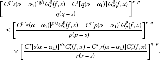
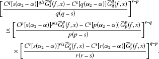
Corollary 2.7 If $s>0$, $p<q<r$ ($p,q,r\in {\mathbb{R}}^{+}$) and $p,q,r\ne s$, then the following inequalities hold:

(24)

(25)

(26)

(27)

Proof For $i=1$, we have

$${\mathcal{L}}_1({\varphi }_p)=\frac{C^p{({\int }_a^{b}f(x)dg(x))}^p-C({\int }_a^b{f}^p(x)d[g^p(x)])}{p(p-1)}.$$

Since $s>0$, so $p/s<q/s<r/s$. Also, for f is C-decreasing, $f^s$ is $C^s$-decreasing. We make substitutions $f\to f^s$, $g\to g^s$, $C\to C^s$, $p\to p/s$, $q\to q/s$, and $r\to r/s$ in (23). We get

$$\begin{array}{rcl}{\left[\frac{C^q{H}_s^q(f,g)-C^s{H}_q^q(f,g)}{\frac{q(q-s)}{s^2}}\right]}^{\frac{r-p}{s}}& \le & {\left[\frac{C^p{H}_s^p(f,g)-C^s{H}_p^p(f,g)}{\frac{p(p-s)}{s^2}}\right]}^{\frac{r-q}{s}}\\ \times {\left[\frac{C^r{H}_s^r(f,g)-C^s{H}_r^r(f,g)}{\frac{r(r-s)}{s^2}}\right]}^{\frac{q-p}{s}}.\end{array}$$

After simplification, we get (24). Similarly, for $i=2,3,4$, we get (25)-(27) respectively. □

Remark 2.8 From the inequalities (24)-(27) for ($q<s$), we get the refinement for inequalities obtained from Theorem 1.2 and reversion when ($q>s$). Of course, we can get such refinement and reversions in all other cases for p, s and r, s.

Corollary 2.9 For $s>0$, $p<q<r$ ($p,q,r\in {\mathbb{R}}^{+}$) and $p,q,r\ne s$.

• (a) If $f\in Q^{{\alpha }_1}(C)$, $\alpha >{\alpha }_1$, then for any $x>0$, the following inequality holds:

  

  (28)

• (b) If $f\in Q_{{\alpha }_2}(C)$, ${\alpha }_2>\alpha$, then for any $x\ge 0$, the following inequality holds:

  

  (29)

Proof (a) It is a simple consequence of Corollary 2.7. Since $f\in Q^{{\alpha }_1}(C)$, by making substitutions $f\to f(t)t^{-{\alpha }_1}$ and $g\to t^{({\alpha }_1-\alpha )}$ in (26), we get (28).

• (b) Since $f\in Q^{{\alpha }_2}(C)$, by making substitutions $f\to f(t)t^{-{\alpha }_2}$ and $g\to t^{({\alpha }_2-\alpha )}$ in (24), we get (29). □

Now, we state and prove the Lagrange-type mean value theorem for the linear functionals ${\mathcal{L}}_i$, $i=1,\dots ,4$ defined by (M₁)-(M₄).

Theorem 2.10 Let ${\mathcal{L}}_i$, $i=1,\dots ,4$ be linear functionals defined by (M₁)-(M₄) and $\varphi \in C^2[0,a]$, $a>0$, such that $\varphi (0)=0$. Then there exists ${\xi }_i\in [0,a]$ such that the identity

$${\mathcal{L}}_i(\varphi )=\frac{{\varphi }^{″}({\xi }_i)}{2}{\mathcal{L}}_i\left(x^2\right)$$

(30)

holds for $i=1,\dots ,4$.

Proof Fix $i=1,\dots ,4$.

Since ${\varphi }^{″}$ is continuous on $[0,a]$, it attains its maximum and minimum value on $[0,a]$. Let

$$m=\underset{x\in [0,a]}{min}\{{\varphi }^{″}(x)\}\text{and}M=\underset{x\in [0,a]}{max}\{{\varphi }^{″}(x)\}.$$

Let us consider functions $F_1,F_2:[0,a]\to \mathbb{R}$ defined by

$$F_1(x)=M\frac{x^2}{2}-\varphi (x)\text{and}{F}_2(x)=\varphi (x)-m\frac{x^2}{2}.$$

Clearly,

$$F_1^{″}(x)=M-{\varphi }^{″}(x)\ge 0,$$

and

$$F_2^{″}(x)={\varphi }^{″}(x)-m\ge 0,$$

so $F_1$, $F_2$ are convex functions. Also, $F_1(0)=0=F_2(0)$. Hence, from Theorem 2.1 for $F_1$ and $F_2$ respectively, it follows

$${\mathcal{L}}_i(\varphi )\le \frac{M}{2}{\mathcal{L}}_i\left(x^2\right)$$

(31)

and

$${\mathcal{L}}_i(\varphi )\ge \frac{m}{2}{\mathcal{L}}_i\left(x^2\right).$$

(32)

Combining (31) and (32), we get

$$\frac{m}{2}{\mathcal{L}}_i\left(x^2\right)\le {\mathcal{L}}_i(\varphi )\le \frac{M}{2}{\mathcal{L}}_i\left(x^2\right).$$

If ${\mathcal{L}}_i(x^2)=0$, then ${\mathcal{L}}_i(\varphi )=0$ and (30) holds for all ${\xi }_i\in [0,a]$. Otherwise,

$$m\le \frac{2{\mathcal{L}}_i(\varphi )}{{\mathcal{L}}_i(x^2)}\le M.$$

Since ${\varphi }^{″}$ is continuous, there exists ${\xi }_i\in [0,a]$ such that (30) holds and the proof is complete. □

Theorem 2.11 Let ${\mathcal{L}}_i$, $i=1,\dots ,4$ be linear functionals defined by (M₁)-(M₄) and $\varphi ,\psi \in C^2[0,a]$, $a>0$, such that $\varphi (0)=0=\psi (0)$. Then there exists ${\xi }_i\in [0,a]$ such that the identity

$$\frac{{\mathcal{L}}_i(\varphi )}{{\mathcal{L}}_i(\psi )}=\frac{{\varphi }^{″}({\xi }_i)}{{\psi }^{″}({\xi }_i)}$$

(33)

holds for $i=1,\dots ,4$, provided that denominators are nonzero.

Proof Fix $1\le i\le 4$ and define $L\in C^2[0,a]$ in the way that

$$L=c_1\varphi -c_2\psi ,$$

where $c_1$ and $c_2$ are defined by $c_1={\mathcal{L}}_i(\psi )$ and $c_2={\mathcal{L}}_i(\varphi )$. Now, from Theorem 2.10 for the function L, it follows

$$(c_1\frac{{\varphi }^{″}({\xi }_i)}{2}-c_2\frac{{\psi }^{″}({\xi }_i)}{2}){\mathcal{L}}_i\left(x^2\right)=0.$$

(34)

Since for (33) the denominators are nonzero, we have ${\mathcal{L}}_i(x^2)\ne 0$ (because if it is zero, then ${\mathcal{L}}_i(\psi )=0$ by Theorem 2.10). Therefore, (34) gives (33). □

Corollary 2.12 Let ${\mathcal{L}}_i$, $i=1,\dots ,4$ be linear functionals defined by (M₁)-(M₄). For distinct positive real numbers l and r different from one, there exists ${\xi }_i\in [0,a]$ such that

$${\xi }_i^{l-r}=\frac{r(r-1){\mathcal{L}}_i(x^l)}{l(l-1){\mathcal{L}}_i(x^r)}$$

(35)

holds for $i=1,\dots ,4$.

Proof Taking $\varphi (x)=x^l$ and $\psi (x)=x^r$ in (33), for distinct positive real numbers l and r different from one, we obtain (35). □

Remark 2.13 Since for fix $i=1,\dots ,4$ the function ${\xi }_i\to {\xi }_i^{l-r}$, $l\ne r$ is invertible, then from (35) we get

$$m\le {\left(\frac{r(r-1){\mathcal{L}}_i(x^l)}{l(l-1){\mathcal{L}}_i(x^r)}\right)}^{\frac{1}{l-r}}\le M,r\ne l,r,l\ne 1.$$

(36)

3 Cauchy means

In this section we deduce Cauchy means from Theorem 2.11. Suppose that ${\varphi }^{″}/{\psi }^{″}$ has inverse. Then (33) gives

$${\xi }_i={\left(\frac{{\varphi }^{″}}{{\psi }^{″}}\right)}^{-1}\left(\frac{{\mathcal{L}}_i(\varphi )}{{\mathcal{L}}_i(\psi )}\right).$$

(37)

We conclude that the expression on the right-hand side of the above equation is also a mean. For $r,l\in {\mathbb{R}}^{+}$, we define the Cauchy means

$$M_{l,r}^i={\left(\frac{r(r-1){\mathcal{L}}_i(x^l)}{l(l-1){\mathcal{L}}_i(x^r)}\right)}^{\frac{1}{l-r}},r\ne l,r,l\ne 1.$$

(38)

Also, we have continuous extensions of these means in other cases. Therefore, by limit, we have the following:

(39)

(40)

(41)

(42)

We also need the following result (see, e.g., [5]).

Lemma 3.1 If Φ is a convex function on an interval $I\subset \mathbb{R}$ and if $r\le u$, $l\le v$, $r\ne l$, $u\ne v$, then the following inequality is valid:

$$\frac{\mathrm{\Phi }(l)-\mathrm{\Phi }(r)}{l-r}\le \frac{\mathrm{\Phi }(v)-\mathrm{\Phi }(u)}{v-u}.$$

(43)

Now, we deduce the monotonicity of means defined by (38) in the form of Dresher’s inequality as follows.

Theorem 3.2 Let $M_{l,r}^i$ be given as in (38) and $r,l,u,v\in {\mathbb{R}}^{+}$ be such that $l\le v$, $r\le u$. Then

$$M_{l,r}^i\le M_{v,u}^i,i=1,\dots ,4.$$

(44)

Proof By Theorem 2.6, ${\mathcal{L}}_i$ is log-convex. We set $\mathrm{\Phi }(l)=log{\mathcal{L}}_i({\varphi }_l)$ in Lemma 3.1 and get

$$\frac{log{\mathcal{L}}_i({\varphi }_l)-log{\mathcal{L}}_i({\varphi }_r)}{l-r}\le \frac{log{\mathcal{L}}_i({\varphi }_v)-log{\mathcal{L}}_i({\varphi }_u)}{v-u}.$$

(45)

By using the properties of a log function, we get immediately (44). □

Corollary 3.3 For distinct positive real numbers l, r and s, there exist ${\xi }_i\in [0,a]$, $i=1,\dots ,4$ such that the following identities hold:

(46)

(47)

(48)

(49)

Proof For $i=1$, making substitutions $f\to f^s$, $g\to g^s$, $C\to C^s$, $\varphi (x)=x^{l/s}$, and $\psi (x)=x^{r/s}$ in (33), we get (46).

Similarly, for $i=2,3,4$, making substitutions as above in (33), we get (47), (48) and (49) respectively. □

Remark 3.4 Since the function ${\xi }_i\to {\xi }_i^{l-r}$ is invertible for all $i=1,\dots ,4$, from (46)-(49), we can again formulate the corresponding Cauchy means for distinct positive real numbers l, r and s.

They are given as follows:

(50)

(51)

(52)

(53)

Corollary 3.5 Let $M_{l,r,s}^i$, $i=1,\dots ,4$ be given as above and $r,l,u,v;s\in {\mathbb{R}}^{+}$ be such that $l\le v$, $r\le u$. Then

$$M_{l,r,s}^i\le M_{v,u,s}^i,i=1,\dots ,4.$$

(54)

Proof By Theorem 3.2,

$$M_{l,r}^i\le M_{v,u}^i,i=1,\dots ,4.$$

For $s>0$, we set $f\to f^s$, $g\to g^s$, $C\to C^s$, $l\to l/s$, $r\to r/s$, $u\to v/s$ and $r\to v/s$ in the above inequality for means and get (54). □

References

Heinig H, Maligranda L: Weighted inequalities for monotone and concave functions. Stud. Math. 1995, 116(2):133–165.
Pečarić J, Perić I, Persson LE: Integral inequalities for monotone functions. J. Math. Anal. Appl. 1997, 215: 235–251. Article No. AY975646 10.1006/jmaa.1997.5646
Anwar M, Pečarić J: On logarithmic-convexity for differences of power means and related results. Math. Inequal. Appl. 2009, 12(1):81–90.
Anwar M, Pečarić J: Means of the Cauchy Type. LAP Lambert Academic Publishing, Saarbrücken; 2009.
Pečarić J, Proschan F, Tong YL Mathematics in Science and Engineering 187. In Convex Functions, Partial Orderings and Statistical Applications. Academic Press, Boston; 1992.
Acknowledgements
The authors wish to thank the anonymous referees for their very careful reading of the manuscript and fruitful comments and suggestions. This research was partially funded by Higher Education Commission, Pakistan. The research of the second author was supported by the Croatian Ministry of Science, Education and Sports under the Research Grant 117-1170889-0888.
Author information
Authors and Affiliations
Corresponding author
Additional information
Competing interests
The authors declare that they have no competing interests.
Authors’ contributions
All authors jointly worked on the results and they read and approved the final manuscript.
Rights and permissions
Open Access This article is distributed under the terms of the Creative Commons Attribution 2.0 International License (https://creativecommons.org/licenses/by/2.0), which permits unrestricted use, distribution, and reproduction in any medium, provided the original work is properly cited.
About this article
Cite this article
Butt, S.I., Pečarić, J. & Perić, I. Refinement of integral inequalities for monotone functions. J Inequal Appl 2012, 301 (2012). https://doi.org/10.1186/1029-242X-2012-301
Received:
Accepted:
Published:
DOI: https://doi.org/10.1186/1029-242X-2012-301