A relation between Hilbert and Carlson inequalities

Abstract

In this paper, we introduce some new inequalities with a best constant factor. As an application, we obtain a sharper form of Hilbert’s inequality. Some inequalities of Carlson type are also considered.

MSC:26D15.

1 Introduction

If $f(x),g(x)\ge 0$, $0<{\int }_0^{\mathrm{\infty }}{f}^2(x)dx<\mathrm{\infty }$, and $0<{\int }_0^{\mathrm{\infty }}{g}^2(x)dx<\mathrm{\infty }$, then (see [1])

$${\int }_0^{\mathrm{\infty }}{\int }_0^{\mathrm{\infty }}\frac{f(x)g(y)}{x+y}dxdy<\pi {\{{\int }_0^{\mathrm{\infty }}{f}^2(x)dx\}}^{\frac{1}{2}}{\{{\int }_0^{\mathrm{\infty }}{g}^2(x)dx\}}^{\frac{1}{2}}.$$

(1.1)

Inequality (1.1) is called Hilbert’s integral inequality, which has been extended by Hardy [1] as: if $p>1$, $\frac{1}{p}+\frac{1}{q}=1$, $f(x),g(x)>0$, $0<{\int }_0^{\mathrm{\infty }}{f}^p(x)dx<\mathrm{\infty }$, and $0<{\int }_0^{\mathrm{\infty }}{g}^q(x)dx<\mathrm{\infty }$, then

$${\int }_0^{\mathrm{\infty }}{\int }_0^{\mathrm{\infty }}\frac{f(x)g(y)}{x+y}dxdy<\frac{\pi }{sin\frac{\pi }{p}}{\{{\int }_0^{\mathrm{\infty }}{f}^p(x)dx\}}^{\frac{1}{p}}{\{{\int }_0^{\mathrm{\infty }}{g}^q(x)dx\}}^{\frac{1}{q}}.$$

(1.2)

The corresponding inequalities in the discrete case are ($a_m,b_n>0$):

(1.3)

(1.4)

provided that the series on the right-hand side of (1.3) and (1.4) are convergent. The constant factor π is the best possible in both (1.1) and (1.3), and the constant $\frac{\pi }{sin\frac{\pi }{p}}$ is the best possible in (1.2) and (1.4). The following general inequality was given in [2]:

(1.5)

where $k(p{A}_2)={\int }_0^{\mathrm{\infty }}K(1,t)t^{-p{A}_2}dt$ is the best possible constant, $K(x,y)\ge 0$ is a homogeneous function of degree −λ ($\lambda >0$), $A_1\in (\frac{1-\lambda }{q},\frac{1}{q})$, $A_2\in (\frac{1-\lambda }{p},\frac{1}{p})$, and $p{A}_2+q{A}_1=2-\lambda$. Moreover, in [3] the following is proved:

$$\sum _{n=1}^{\mathrm{\infty }}\sum _{m=1}^{\mathrm{\infty }}K(m,n)a_m{b}_n<k(p{A}_2){\left\{\sum _{n=1}^{\mathrm{\infty }}{m}^{pq{A}_1-1}{a}_m^p\right\}}^{\frac{1}{p}}{\left\{\sum _{n=1}^{\mathrm{\infty }}{n}^{pq{A}_2-1}{b}_n^q\right\}}^{\frac{1}{q}},$$

(1.6)

here $K(x,y)\ge 0$ is a homogeneous function of degree −λ ($\lambda >0$) strictly decreasing in both parameters x and y, $A_1\in (max\{\frac{1-\lambda }{q},0\},\frac{1}{q})$, $A_2\in (max\{\frac{1-\lambda }{p},0\},\frac{1}{p})$, and $p{A}_2+q{A}_1=2-\lambda$. In particular, if we set $K(x,y)=\frac{1}{\alpha x+\beta y}$ and $K(m,n)=\frac{1}{\alpha m+\beta n}$ ($\alpha ,\beta >0$) respectively in (1.5) and (1.6) for $\lambda =1$, we have

(1.7)

(1.8)

where $B(s,t)$ is the beta function, $A_1\in (0,\frac{1}{q})$, $A_2\in (0,\frac{1}{p})$, and $p{A}_2+q{A}_1=1$. We need the following formula for the beta function:

$$B(s,t+1)=\frac{t}{s+t}B(s,t).$$

(1.9)

For the sequence of real numbers $(a_n)$, Carlson’s inequality is given as

$$\sum _{n=1}^{\mathrm{\infty }}{a}_n<\sqrt{\pi }{\left(\sum _{n=1}^{\mathrm{\infty }}{a}_n^2\right)}^{\frac{1}{4}}{\left(\sum _{n=1}^{\mathrm{\infty }}{n}^2{a}_n^2\right)}^{\frac{1}{4}},$$

(1.10)

the constant $\sqrt{\pi }$ is the best possible. The continuous version of (1.10) is

$${\int }_0^{\mathrm{\infty }}f(x)dx\le \sqrt{\pi }{({\int }_0^{\mathrm{\infty }}{f}^2(x)dx)}^{\frac{1}{4}}{({\int }_0^{\mathrm{\infty }}{x}^2{f}^2(x)dx)}^{\frac{1}{4}},$$

(1.11)

the constant $\sqrt{\pi }$ is sharp. Regarding these inequalities and their extensions, we refer the reader to the book [4].

In this paper, we introduce two new inequalities with a best constant factor which gives an upper estimate for the double series ${\sum }_{n=1}^{\mathrm{\infty }}{\sum }_{m=1}^{\mathrm{\infty }}{\sigma }_{n,m}$ and the double integral ${\int }_0^{\mathrm{\infty }}{\int }_0^{\mathrm{\infty }}G(x,y)dxdy$, where ${\sigma }_{n,m}$ is a double sequence of positive numbers and $G(x,y)$ is a positive function on $(0,\mathrm{\infty })\times (0,\mathrm{\infty })$. As an application, we obtain a sharper form of the Hilbert inequality. Some examples of Carlson type inequalities are also considered. The proof of the inequalities depends on inequalities (1.7), (1.8) and Hardy’s idea in proving Carlson’s inequality.

2 Discrete case

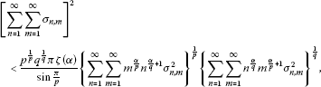
Theorem 2.1 Let $p>1$, $\frac{1}{p}+\frac{1}{q}=1$, $a_n$ and $b_n$ be two sequences of positive numbers such that $0<{\sum }_{m=1}^{\mathrm{\infty }}{m}^{pq{A}_1-1}{a}_m^p<\mathrm{\infty }$, $0<{\sum }_{n=1}^{\mathrm{\infty }}{n}^{pq{A}_2-1}{b}_n^q<\mathrm{\infty }$. Let ${\sigma }_{n,m}$ be a double sequence of positive numbers such that ${\sum }_{n=1}^{\mathrm{\infty }}{\sum }_{m=1}^{\mathrm{\infty }}\frac{m{\sigma }_{n,m}^2}{a_m{b}_n}<\mathrm{\infty }$ and ${\sum }_{n=1}^{\mathrm{\infty }}{\sum }_{m=1}^{\mathrm{\infty }}\frac{n{\sigma }_{n,m}^2}{a_m{b}_n}<\mathrm{\infty }$, then the following inequality holds:

$$\begin{array}{rcl}{\left[\sum _{n=1}^{\mathrm{\infty }}\sum _{m=1}^{\mathrm{\infty }}{\sigma }_{n,m}\right]}^2& <& L{\left\{\sum _{m=1}^{\mathrm{\infty }}{m}^{pq{A}_1-1}{a}_m^p\right\}}^{\frac{1}{p}}{\left\{\sum _{n=1}^{\mathrm{\infty }}{n}^{pq{A}_2-1}{b}_n^q\right\}}^{\frac{1}{q}}\\ \times {\left\{\sum _{n=1}^{\mathrm{\infty }}\sum _{m=1}^{\mathrm{\infty }}\frac{n{\sigma }_{n,m}^2}{a_m{b}_n}\right\}}^{q{A}_1}{\left\{\sum _{n=1}^{\mathrm{\infty }}\sum _{m=1}^{\mathrm{\infty }}\frac{m{\sigma }_{n,m}^2}{a_m{b}_n}\right\}}^{p{A}_2},\end{array}$$

(2.1)

here $A_1\in (0,\frac{1}{q})$, $A_2\in (0,\frac{1}{p})$, $p{A}_2+q{A}_1=1$, and the constant $L=\frac{B(p{A}_2,1-p{A}_2)}{{(p{A}_2)}^{p{A}_2}{(q{A}_1)}^{q{A}_1}}$ is the best possible.

Proof Let $\alpha ,\beta >0$, using Cauchy’s inequality and then applying (1.8), we get

$$\begin{array}{rcl}{\left[\sum _{n=1}^{\mathrm{\infty }}\sum _{m=1}^{\mathrm{\infty }}{\sigma }_{n,m}\right]}^2& =& {\left[\sum _{n=1}^{\mathrm{\infty }}\sum _{m=1}^{\mathrm{\infty }}\left\{\frac{\sqrt{a_m{b}_n}}{\sqrt{\alpha m+\beta n}}\right\}\left\{\frac{\sqrt{\alpha m+\beta n}}{\sqrt{a_m{b}_n}}{\sigma }_{n,m}\right\}\right]}^2\\ \le & \sum _{n=1}^{\mathrm{\infty }}\sum _{m=1}^{\mathrm{\infty }}\frac{a_m{b}_n}{\alpha m+\beta n}\sum _{n=1}^{\mathrm{\infty }}\sum _{m=1}^{\mathrm{\infty }}\frac{\alpha m+\beta n}{a_m{b}_n}{\sigma }_{n,m}^2\\ <& \frac{B(p{A}_2,1-p{A}_2)}{{\alpha }^{1-q{A}_1}{\beta }^{1-p{A}_2}}{\left\{\sum _{m=1}^{\mathrm{\infty }}{m}^{pq{A}_1-1}{a}_m^p\right\}}^{\frac{1}{p}}{\left\{\sum _{n=1}^{\mathrm{\infty }}{n}^{pq{A}_2-1}{b}_n^q\right\}}^{\frac{1}{q}}\\ \times [\alpha \sum _{n=1}^{\mathrm{\infty }}\sum _{m=1}^{\mathrm{\infty }}\frac{m{\sigma }_{n,m}^2}{a_m{b}_n}+\beta \sum _{n=1}^{\mathrm{\infty }}\sum _{m=1}^{\mathrm{\infty }}\frac{n{\sigma }_{n,m}^2}{a_m{b}_n}]\\ =& B(p{A}_2,1-p{A}_2){\left\{\sum _{m=1}^{\mathrm{\infty }}{m}^{pq{A}_1-1}{a}_m^p\right\}}^{\frac{1}{p}}{\left\{\sum _{n=1}^{\mathrm{\infty }}{n}^{pq{A}_2-1}{b}_n^q\right\}}^{\frac{1}{q}}\\ \times [{\left(\frac{\alpha }{\beta }\right)}^{q{A}_1}\sum _{n=1}^{\mathrm{\infty }}\sum _{m=1}^{\mathrm{\infty }}\frac{m{\sigma }_{n,m}^2}{a_m{b}_n}+{\left(\frac{\beta }{\alpha }\right)}^{p{A}_2}\sum _{n=1}^{\mathrm{\infty }}\sum _{m=1}^{\mathrm{\infty }}\frac{n{\sigma }_{n,m}^2}{a_m{b}_n}].\end{array}$$

Set $T={\sum }_{n=1}^{\mathrm{\infty }}{\sum }_{m=1}^{\mathrm{\infty }}\frac{m{\sigma }_{n,m}^2}{a_m{b}_n}$, $S={\sum }_{n=1}^{\mathrm{\infty }}{\sum }_{m=1}^{\mathrm{\infty }}\frac{n{\sigma }_{n,m}^2}{a_m{b}_n}$, $t=\frac{\alpha }{\beta }$ and consider the function $h(t)=t^{q{A}_1}T+t^{-p{A}_2}S$. Since $h^{\mathrm{\prime }}(t)=\frac{1}{t^{p{A}_2}}(q{A}_{1}T-\frac{p{A}_{2}S}{t})$, we conclude that the minimum of this function attains for $t=\frac{p{A}_{2}S}{q{A}_{1}T}$. Therefore, if we let $\alpha =p{A}_{2}S$ and $\beta =q{A}_{1}T$, we get (2.1).

It remains to show that the constant L in (2.1) is the best possible. To do that, suppose that there exists a positive constant $C<L$ such that (2.1) is still valid if we replace L by C. For $0<\epsilon <q(1-p{A}_2)$, setting ${\tilde{a}}_m$ and ${\tilde{b}}_n$ as ${\tilde{a}}_m=m^{-q{A}_1-\frac{\epsilon }{p}}$, $\widetilde{b_n}=n^{-p{A}_2-\frac{\epsilon }{q}}$, and ${\tilde{\sigma }}_{n,m}=\frac{{\tilde{a}}_m{\tilde{b}}_n}{m+n}$, we have ${\sum }_{m=1}^{\mathrm{\infty }}{m}^{pq{A}_1-1}{\tilde{a}}_m^p={\sum }_{m=1}^{\mathrm{\infty }}\frac{1}{m^{1+\epsilon }}=1+{\sum }_{m=2}^{\mathrm{\infty }}\frac{1}{m^{1+\epsilon }}<1+{\int }_1^{\mathrm{\infty }}{x}^{-1-\epsilon }dx=1+\frac{1}{\epsilon }$; similarly, we obtain ${\sum }_{n=1}^{\mathrm{\infty }}{n}^{pq{A}_2-1}{\tilde{b}}_n^q<1+\frac{1}{\epsilon }$. Moreover,

$$\begin{array}{rcl}\sum _{n=1}^{\mathrm{\infty }}\sum _{m=1}^{\mathrm{\infty }}\frac{n{\tilde{\sigma }}_{n,m}^2}{{\tilde{a}}_m{\tilde{b}}_n}& =& \sum _{n=1}^{\mathrm{\infty }}{n}^{1-p{A}_2-\frac{\epsilon }{q}}\sum _{m=1}^{\mathrm{\infty }}\frac{m^{-q{A}_1-\frac{\epsilon }{p}}}{{(m+n)}^2}\\ <& \sum _{n=1}^{\mathrm{\infty }}{n}^{1-p{A}_2-\frac{\epsilon }{q}}{\int }_0^{\mathrm{\infty }}\frac{x^{-q{A}_1-\frac{\epsilon }{p}}}{{(n+x)}^2}dx\\ =& \sum _{n=1}^{\mathrm{\infty }}{n}^{-1-\epsilon }{\int }_0^{\mathrm{\infty }}\frac{u^{-q{A}_1-\frac{\epsilon }{p}}}{{(1+u)}^2}du=[B(1-q{A}_1,1+q{A}_1)+o(1)]\sum _{n=1}^{\mathrm{\infty }}{n}^{-1-\epsilon }\\ <& \frac{\epsilon +1}{\epsilon }[B(1-q{A}_1,1+q{A}_1)+o(1)].\end{array}$$

Similarly,

$$\begin{array}{rcl}\sum _{n=1}^{\mathrm{\infty }}\sum _{m=1}^{\mathrm{\infty }}\frac{m{\tilde{\sigma }}_{n,m}^2}{{\tilde{a}}_m{\tilde{b}}_n}& =& \sum _{m=1}^{\mathrm{\infty }}{m}^{1-q{A}_1-\frac{\epsilon }{p}}\sum _{n=1}^{\mathrm{\infty }}\frac{m^{-p{A}_2-\frac{\epsilon }{q}}}{{(m+n)}^2}<\sum _{m=1}^{\mathrm{\infty }}{m}^{1-q{A}_1-\frac{\epsilon }{p}}{\int }_0^{\mathrm{\infty }}\frac{x^{-p{A}_2-\frac{\epsilon }{q}}}{{(m+x)}^2}dx\\ =& \sum _{m=1}^{\mathrm{\infty }}{m}^{-1-\epsilon }{\int }_0^{\mathrm{\infty }}\frac{u^{-p{A}_2-\frac{\epsilon }{q}}}{{(1+u)}^2}du=[B(1-p{A}_2,1+p{A}_2)+o(1)]\sum _{m=1}^{\mathrm{\infty }}{m}^{-1-\epsilon }\\ <& \frac{\epsilon +1}{\epsilon }[B(1-p{A}_2,1+p{A}_2)+o(1)].\end{array}$$

On the other hand,

$$\begin{array}{rcl}\sum _{n=1}^{\mathrm{\infty }}\sum _{m=1}^{\mathrm{\infty }}{\tilde{\sigma }}_{n,m}& =& \sum _{n=1}^{\mathrm{\infty }}\sum _{m=1}^{\mathrm{\infty }}\frac{m^{-q{A}_1-\frac{\epsilon }{p}}{n}^{-p{A}_2-\frac{\epsilon }{q}}}{m+n}>{\int }_1^{\mathrm{\infty }}{\int }_1^{\mathrm{\infty }}\frac{x^{-q{A}_1-\frac{\epsilon }{p}}{y}^{-p{A}_2-\frac{\epsilon }{q}}}{x+y}dxdy\\ >& \frac{1}{\epsilon }[B(p{A}_2,1-p{A}_2)+o(1)]-O(1).\end{array}$$

Substituting the above inequalities in (2.1), we get

(2.2)

Multiplying inequality (2.2) by ${\epsilon }^2$ ($\epsilon ={\epsilon }^{q{A}_1}{\epsilon }^{p{A}_2}$) and then letting $\epsilon \to 0^{+}$, we have

$$B^2(p{A}_2,1-p{A}_2)\le C{B}^{q{A}_1}(1-q{A}_1,1+q{A}_1)B^{p{A}_2}(1-p{A}_2,1+p{A}_2).$$

(2.3)

Using (1.9), we find

$$\begin{array}{rcl}{B}^{q{A}_1}(1-q{A}_1,1+q{A}_1)& =& {(q{A}_1)}^{q{A}_1}{B}^{q{A}_1}(1-q{A}_1,q{A}_1)\\ =& {(q{A}_1)}^{q{A}_1}{B}^{q{A}_1}(p{A}_2,1-p{A}_2),\end{array}$$

(2.4)

and

$$B^{p{A}_2}(1-p{A}_2,1+p{A}_2)={(p{A}_2)}^{p{A}_2}{B}^{p{A}_2}(1-p{A}_2,p{A}_2).$$

(2.5)

Substituting (2.4) and (2.5) in (2.3), we obtain the contradiction $C\ge L=\frac{B(p{A}_2,1-p{A}_2)}{{(p{A}_2)}^{p{A}_2}{(q{A}_1)}^{q{A}_1}}$. The theorem is proved. □

2.1 Some applications

• 1. If ${\sigma }_{n,m}=\frac{a_m{b}_n}{m+n}$ in (2.1), then we have the following form of Hilbert’s inequality:

  $$\begin{array}{rcl}\sum _{n=1}^{\mathrm{\infty }}\sum _{m=1}^{\mathrm{\infty }}\frac{a_m{b}_n}{m+n}& <& \sqrt{L}{\left\{\sum _{m=1}^{\mathrm{\infty }}{m}^{pq{A}_1-1}{a}_m^p\right\}}^{\frac{1}{2p}}{\left\{\sum _{n=1}^{\mathrm{\infty }}{n}^{pq{A}_2-1}{b}_n^q\right\}}^{\frac{1}{2q}}\\ \times {\left\{\sum _{n=1}^{\mathrm{\infty }}\sum _{m=1}^{\mathrm{\infty }}\frac{n{a}_m{b}_n}{{(m+n)}^2}\right\}}^{\frac{q{A}_1}{2}}{\left\{\sum _{n=1}^{\mathrm{\infty }}\sum _{m=1}^{\mathrm{\infty }}\frac{m{a}_m{b}_n}{{(m+n)}^2}\right\}}^{\frac{p{A}_2}{2}}.\end{array}$$

  (2.6)

Inequality (2.6) is a sharper form of (1.8). To see that, let us rewrite (2.6) in the following form:

$${\left\{\sum _{n=1}^{\mathrm{\infty }}\sum _{m=1}^{\mathrm{\infty }}\frac{a_m{b}_n}{m+n}\right\}}^2<\frac{B(p{A}_2,1-p{A}_2)}{{(p{A}_2)}^{p{A}_2}{(q{A}_1)}^{q{A}_1}}{\left\{\sum _{m=1}^{\mathrm{\infty }}{m}^{pq{A}_1-1}{a}_m^p\right\}}^{\frac{1}{p}}{\left\{\sum _{n=1}^{\mathrm{\infty }}{n}^{pq{A}_2-1}{b}_n^q\right\}}^{\frac{1}{q}}{S}^{q{A}_1}{T}^{p{A}_2},$$

where $S={\sum }_{n=1}^{\mathrm{\infty }}{\sum }_{m=1}^{\mathrm{\infty }}\frac{n{a}_m{b}_n}{{(m+n)}^2}$ and $T={\sum }_{n=1}^{\mathrm{\infty }}{\sum }_{m=1}^{\mathrm{\infty }}\frac{m{a}_m{b}_n}{{(m+n)}^2}$. Since we may write ${\sum }_{n=1}^{\mathrm{\infty }}{\sum }_{m=1}^{\mathrm{\infty }}\frac{a_m{b}_n}{m+n}=T+S$, dividing both sides of the last inequality by ${\sum }_{n=1}^{\mathrm{\infty }}{\sum }_{m=1}^{\mathrm{\infty }}\frac{a_m{b}_n}{m+n}$, we get

$$\begin{array}{rcl}\sum _{n=1}^{\mathrm{\infty }}\sum _{m=1}^{\mathrm{\infty }}\frac{a_m{b}_n}{m+n}& <& B(p{A}_2,1-p{A}_2){\left\{\sum _{m=1}^{\mathrm{\infty }}{m}^{pq{A}_1-1}{a}_m^p\right\}}^{\frac{1}{p}}{\left\{\sum _{n=1}^{\mathrm{\infty }}{n}^{pq{A}_2-1}{b}_n^q\right\}}^{\frac{1}{q}}\\ \times \frac{{(\frac{S}{q{A}_1})}^{q{A}_1}{(\frac{T}{p{A}_2})}^{p{A}_2}}{T+S}.\end{array}$$

(2.7)

Applying Young’s inequality ($x^{\theta }{y}^{\mu }\le \theta x+\mu y$, $\theta +\mu =1$) to the product ${(\frac{S}{q{A}_1})}^{q{A}_1}{(\frac{T}{p{A}_2})}^{p{A}_2}$ with $x=\frac{S}{q{A}_1}$ and $y=\frac{T}{p{A}_2}$, we obtain

$$\frac{{(\frac{S}{q{A}_1})}^{q{A}_1}{(\frac{T}{p{A}_2})}^{p{A}_2}}{T+S}\le \frac{T+S}{T+S}=1.$$

Therefore, inequality (2.6) is a sharper form of (1.8). In particular, if we set $p=q=2$, $A_1=\frac{1}{4}=A_2$ in (2.6), we obtain the following sharper form of the classical Hilbert inequality (1.3):

$$\begin{array}{rcl}{\left[\sum _{n=1}^{\mathrm{\infty }}\sum _{m=1}^{\mathrm{\infty }}\frac{a_m{b}_n}{m+n}\right]}^2& <& 2\pi {\left\{\sum _{m=1}^{\mathrm{\infty }}{a}_m^2\right\}}^{\frac{1}{2}}{\left\{\sum _{n=1}^{\mathrm{\infty }}{b}_n^2\right\}}^{\frac{1}{2}}\\ \times {\left\{\sum _{n=1}^{\mathrm{\infty }}\sum _{m=1}^{\mathrm{\infty }}\frac{n{a}_m{b}_n}{{(m+n)}^2}\right\}}^{\frac{1}{2}}{\left\{\sum _{n=1}^{\mathrm{\infty }}\sum _{m=1}^{\mathrm{\infty }}\frac{m{a}_m{b}_n}{{(m+n)}^2}\right\}}^{\frac{1}{2}}.\end{array}$$

(2.8)

Note that we may obtain the Hilbert inequality from (2.8) by applying the AG inequality $\sqrt{ST}\le \frac{S+T}{2}$ to the right-hand side of (2.8).

• 2. The more accurate Hilbert inequality is given as

  $$\sum _{n=1}^{\mathrm{\infty }}\sum _{m=1}^{\mathrm{\infty }}\frac{a_m{b}_n}{m+n+1}<\frac{\pi }{sin\frac{\pi }{p}}{\left\{\sum _{n=1}^{\mathrm{\infty }}{a}_n^p\right\}}^{\frac{1}{p}}{\left\{\sum _{n=1}^{\mathrm{\infty }}{b}_n^q\right\}}^{\frac{1}{q}}.$$

  (2.9)

If we put ${\sigma }_{n,m}=\frac{a_m{b}_n}{m+n+\mu }$ ($\mu >0$) in (2.1), then we have

Since

we obtain

$$\begin{array}{rcl}\sum _{n=1}^{\mathrm{\infty }}\sum _{m=1}^{\mathrm{\infty }}\frac{a_m{b}_n}{m+n+\mu }& <& B(p{A}_2,1-p{A}_2){\left\{\sum _{m=1}^{\mathrm{\infty }}{m}^{pq{A}_1-1}{a}_m^p\right\}}^{\frac{1}{p}}{\left\{\sum _{n=1}^{\mathrm{\infty }}{n}^{pq{A}_2-1}{b}_n^q\right\}}^{\frac{1}{q}}\\ \times \frac{{(\frac{S_1}{q{A}_1})}^{q{A}_1}{(\frac{S_2}{p{A}_2})}^{p{A}_2}}{S_1+S_2+S_3}.\end{array}$$

Applying Young’s inequality, we get $\frac{{(\frac{S_1}{q{A}_1})}^{q{A}_1}{(\frac{S_2}{p{A}_2})}^{p{A}_2}}{S_1+S_2+S_3}\le \frac{S_1+S_2}{S_1+S_2+S_3}<1$, thus we arrive at

$$\sum _{n=1}^{\mathrm{\infty }}\sum _{m=1}^{\mathrm{\infty }}\frac{a_m{b}_n}{m+n+\mu }<B(p{A}_2,1-p{A}_2){\left\{\sum _{m=1}^{\mathrm{\infty }}{m}^{pq{A}_1-1}{a}_m^p\right\}}^{\frac{1}{p}}{\left\{\sum _{n=1}^{\mathrm{\infty }}{n}^{pq{A}_2-1}{b}_n^q\right\}}^{\frac{1}{q}}.$$

In particular, if $\mu =1$, $A_1=\frac{1}{pq}=A_2$, then we have (2.9).

• 3. For $\alpha >1$, set $a_m=m^{-\frac{\alpha }{p}}$, $b_n=n^{-\frac{\alpha }{q}}$, and $A_1=A_2=\frac{1}{pq}$ in (2.1), then we get

  

where $\zeta (\alpha )$ is the Riemann zeta function. In particular, if $\alpha =2$ and if ${\sigma }_{n,m}=c_m{c}_n$, then we get the following Carlson type inequality:

$$\sum _{m=1}^{\mathrm{\infty }}{c}_m<{\left(\frac{{\pi }^3}{3}\right)}^{\frac{1}{4}}{\left\{\sum _{m=1}^{\mathrm{\infty }}m{c}_m^2\right\}}^{\frac{1}{4}}{\left\{\sum _{m=1}^{\mathrm{\infty }}{m}^2{c}_m^2\right\}}^{\frac{1}{4}}.$$

• 4. If we let ${\sigma }_{n,m}=a_m{a}_n$ and $b_n=a_n$, $p=q=2$, $A_1=A_2=\frac{1}{4}$, we get

  $$\sum _{m=1}^{\mathrm{\infty }}{a}_m<{(2\pi )}^{\frac{1}{3}}{\left\{\sum _{m=1}^{\mathrm{\infty }}m{a}_m\right\}}^{\frac{1}{3}}{\left\{\sum _{m=1}^{\mathrm{\infty }}{a}_m^2\right\}}^{\frac{1}{3}}.$$

3 Integral case

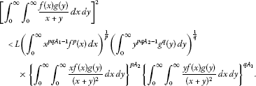
Theorem 3.1 If $p>1$, $\frac{1}{p}+\frac{1}{q}=1$, $f(x),g(x)>0$ such that $0<{\int }_0^{\mathrm{\infty }}{x}^{pq{A}_1-1}{f}^p(x)dx<\mathrm{\infty }$, $0<{\int }_0^{\mathrm{\infty }}{x}^{pq{A}_1-1}{g}^q(x)dx<\mathrm{\infty }$, suppose also that the function $G(x,y)$ is positive on $(0,\mathrm{\infty })\times (0,\mathrm{\infty })$ and that ${\int }_0^{\mathrm{\infty }}{\int }_0^{\mathrm{\infty }}\frac{x{G}^2(x,y)}{f(x)g(y)}dxdy<\mathrm{\infty }$, ${\int }_0^{\mathrm{\infty }}{\int }_0^{\mathrm{\infty }}\frac{y{G}^2(x,y)}{f(x)g(y)}dxdy<\mathrm{\infty }$, then the following inequality holds:

(3.1)

where $A_1\in (0,\frac{1}{q})$, $A_2\in (0,\frac{1}{p})$, $p{A}_2+q{A}_1=1$, and the constant $L=\frac{B(p{A}_2,1-p{A}_2)}{{(p{A}_2)}^{p{A}_2}{(q{A}_1)}^{q{A}_1}}$ is the best possible.

Proof By Cauchy’s inequality, taking into account (1.7), we get ($\alpha ,\beta >0$)

As in the proof of Theorem 2.1, if we set $I_1={\int }_0^{\mathrm{\infty }}{\int }_0^{\mathrm{\infty }}\frac{x{G}^2(x,y)}{f(x)g(y)}dxdy$, $I_2={\int }_0^{\mathrm{\infty }}{\int }_0^{\mathrm{\infty }}\frac{y{G}^2(x,y)}{f(x)g(y)}dxdy$, $t=\frac{\alpha }{\beta }$ and consider the function $h(t)=t^{q{A}_1}{I}_1+t^{-p{A}_2}{I}_2$, we find that the minimum of this function attains for $t=\frac{p{A}_2{I}_2}{q{A}_1{I}_1}$. Thus, if we let $\alpha =p{A}_2{I}_2$ and $\beta =q{A}_1{I}_1$, we get (3.1). If the constant factor L is not the best possible, then there exists a positive constant M (with $M<L$), thus (3.1) is still valid if we replace L by M. For $0<\epsilon <q(1-p{A}_2)$, setting $\tilde{f}$ and $\tilde{g}$ as $\tilde{f}(x)=\tilde{g}(x)=0$ for $x\in (0,1)$, $\tilde{f}(x)=x^{-q{A}_{1-}\frac{\epsilon }{p}}$, $\tilde{g}(x)=x^{-p{A}_{2-}\frac{\epsilon }{q}}$ for $x\in [1,\mathrm{\infty })$, and setting $\tilde{G}(x,y)=\frac{\tilde{f}(x)\tilde{g}(y)}{x+y}$, we have

$$\begin{array}{rcl}{I}^2& :=& {[{\int }_1^{\mathrm{\infty }}{\int }_1^{\mathrm{\infty }}\tilde{G}(x,y)dxdy]}^2\\ <& M{\left({\int }_1^{\mathrm{\infty }}{x}^{-1-\epsilon }dx\right)}^{\frac{1}{p}}{\left({\int }_1^{\mathrm{\infty }}{y}^{-1-\epsilon }dy\right)}^{\frac{1}{q}}{\left\{{\int }_1^{\mathrm{\infty }}{\int }_1^{\mathrm{\infty }}\frac{x^{1-q{A}_1-\frac{\epsilon }{p}}{y}^{-p{A}_{2-}\frac{\epsilon }{q}}}{{(x+y)}^2}dxdy\right\}}^{p{A}_2}\\ \times {\left\{{\int }_1^{\mathrm{\infty }}{\int }_1^{\mathrm{\infty }}\frac{y^{1-p{A}_{2-}\frac{\epsilon }{q}}{x}^{-q{A}_1-\frac{\epsilon }{p}}}{{(x+y)}^2}dxdy\right\}}^{q{A}_1}\\ =& \frac{M}{\epsilon }{(I_1)}^{p{A}_2}{(I_2)}^{q{A}_1}.\end{array}$$

(3.2)

Let $y=ux$, then we have

$$\begin{array}{rcl}{I}_1& =& {\int }_1^{\mathrm{\infty }}{x}^{-1-\epsilon }{\int }_{1/x}^{\mathrm{\infty }}\frac{u^{-p{A}_2-\frac{\epsilon }{q}}}{{(1+u)}^2}dudx<{\int }_1^{\mathrm{\infty }}{x}^{-1-\epsilon }{\int }_0^{\mathrm{\infty }}\frac{u^{-p{A}_2-\frac{\epsilon }{q}}}{{(1+u)}^2}dudx\\ =& \frac{1}{\epsilon }[B(1-p{A}_2,1+p{A}_2)+o(1)].\end{array}$$

Similarly,

$$\begin{array}{rcl}{I}_2& =& {\int }_1^{\mathrm{\infty }}{x}^{-1-\epsilon }{\int }_{1/x}^{\mathrm{\infty }}\frac{u^{1-p{A}_2-\frac{\epsilon }{q}}}{{(1+u)}^2}dudy<{\int }_1^{\mathrm{\infty }}{x}^{-1-\epsilon }{\int }_0^{\mathrm{\infty }}\frac{u^{1-p{A}_2-\frac{\epsilon }{q}}}{{(1+u)}^2}dudx\\ =& \frac{1}{\epsilon }[B(p{A}_2,2-p{A}_2)+o(1)].\end{array}$$

Finally,

$$\begin{array}{rcl}I& =& {\int }_1^{\mathrm{\infty }}{x}^{-1-\epsilon }{\int }_{1/x}^{\mathrm{\infty }}\frac{u^{-p{A}_2-\frac{\epsilon }{q}}}{1+u}dudx\\ >& \frac{1}{\epsilon }[B(1-p{A}_2,p{A}_2)+o(1)]-O(1).\end{array}$$

Substituting the above estimates in (3.2) and then letting $\epsilon \to 0^{+}$, we find $M\ge \frac{B(p{A}_2,1-p{A}_2)}{{\alpha }^{1-q{A}_1}{\beta }^{1-p{A}_2}}$. The theorem is proved. □

3.1 Some applications

• 1. Putting $G(x,y)=\frac{f(x)g(y)}{x+y}$ in inequality (3.1), we get

  

  (3.3)

We may prove that inequality (3.3) is sharper than inequality (1.7) as we did in the discrete case, or we may do that by using (1.5) in the following way: set $K(x,y)=\frac{x}{{(x+y)}^2}$ and $K(x,y)=\frac{y}{{(x+y)}^2}$ respectively in (1.5), then we have

and

Using these two inequalities in (3.3), we get (1.7). In particular, if we set $p=q=2$, $A_1=\frac{1}{4}=A_2$ in (3.3), we obtain the following sharper form of the Hilbert inequality (1.1):

• 2. Assuming $G(x,y)=\frac{f(x)g(y)}{x+y+\mu }$ ($\mu >0$) in inequality (3.1), we get

  

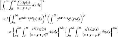
Since we may write ${\int }_0^{\mathrm{\infty }}{\int }_0^{\mathrm{\infty }}\frac{f(x)g(y)}{x+y+\mu }dxdy={\int }_0^{\mathrm{\infty }}{\int }_0^{\mathrm{\infty }}\frac{xf(x)g(y)}{{(x+y+\mu )}^2}dxdy+{\int }_0^{\mathrm{\infty }}{\int }_0^{\mathrm{\infty }}\frac{yf(x)g(y)}{{(x+y+\mu )}^2}dxdy+{\int }_0^{\mathrm{\infty }}{\int }_0^{\mathrm{\infty }}\frac{\mu f(x)g(y)}{{(x+y+\mu )}^2}dxdy=I_1+I_2+I_3$,

the quotient $\frac{{(\frac{I_1}{q{A}_1})}^{q{A}_1}{(\frac{I_2}{p{A}_2})}^{p{A}_2}}{I_1+I_2+I_3}\le 1$, thus we have the following inequality:

• 3. Put $f(x)=e^{-x}$ and $g(y)=e^{-y}$ in (3.1), $A_1=\frac{1}{pq}=A_2$, then we get the following Carlson type inequality for functions of two variables:

  

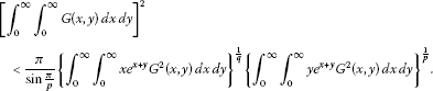  (3.4)

Moreover, if we assume $G(x,y)=\phi (x)\phi (y)$ in (3.4), we get ($p=2$)

$${\int }_0^{\mathrm{\infty }}\phi (x)dx<{\pi }^{\frac{1}{4}}{\{{\int }_0^{\mathrm{\infty }}x{e}^x{\phi }^2(x)dx\}}^{\frac{1}{4}}{\{{\int }_0^{\mathrm{\infty }}{e}^x{\phi }^2(x)dx\}}^{\frac{1}{4}},$$

which is a sharper form of Carlson’s inequality (1.11).

• 4. Let $G(x,y)=f(x)f(y)$, $f(x)=g(x)$ in (3.1), then we obtain the following Carlson type inequality:

  $${\int }_0^{\mathrm{\infty }}f(x)dx<{(2\pi )}^{\frac{1}{3}}{\{{\int }_0^{\mathrm{\infty }}xf(x)dx\}}^{\frac{1}{3}}{\{{\int }_0^{\mathrm{\infty }}{f}^2(x)dx\}}^{\frac{1}{3}}.$$

References

Hardy GH, Littlewood JE, Polya G: Inequalities. Cambridge University Press, London; 1952.
Krnić M, Pecarić J: General Hilbert’s and Hardy’s inequalities. Math. Inequal. Appl. 2005, 8(1):29–52.
Pecarić J, Vuković P: Hardy-Hilbert type inequalities with a homogeneous kernel in discrete form. J. Inequal. Appl. 2010., 2010: Article ID 912601
Larsson L, Maligranda L, Pecarić J, Persson LE: Multiplicative Inequalities of Carlson Type and Interpolation. World Scientific, Hackensack; 2006.
Author information
Authors and Affiliations
Corresponding author
Additional information
Competing interests
The author declares that he has no competing interests.
Rights and permissions
Open Access This article is distributed under the terms of the Creative Commons Attribution 2.0 International License (https://creativecommons.org/licenses/by/2.0), which permits unrestricted use, distribution, and reproduction in any medium, provided the original work is properly cited.
About this article
Cite this article
Azar, L. A relation between Hilbert and Carlson inequalities. J Inequal Appl 2012, 277 (2012). https://doi.org/10.1186/1029-242X-2012-277
Received:
Accepted:
Published:
DOI: https://doi.org/10.1186/1029-242X-2012-277