- Research Article
- Open access
- Published:
Optimality Conditions for Approximate Solutions in Multiobjective Optimization Problems
Journal of Inequalities and Applications volume 2010, Article number: 620928 (2010)
Abstract
We study first- and second-order necessary and sufficient optimality conditions for approximate (weakly, properly) efficient solutions of multiobjective optimization problems. Here, tangent cone,  -normal cone, cones of feasible directions, second-order tangent set, asymptotic second-order cone, and Hadamard upper (lower) directional derivatives are used in the characterizations. The results are first presented in convex cases and then generalized to nonconvex cases by employing local concepts.
1. Introduction
The investigation of the optimality conditions is one of the most attractive topics of optimization theory. For vector optimization, the optimality solutions can be characterized with the help of different geometrical concepts. Miettinen and Mäkelä [1] and Huang and Liu [2] derived several optimality conditions for efficient, weakly efficient, and properly efficient solutions of vector optimization problems with the help of several kinds of cones. Engau and Wiecek [3] derived the cone characterizations for approximate solutions of vector optimization problems by using translated cones. In [4], Aghezzaf and Hachimi obtained second-order optimality conditions by means of a second-order tangent set which can be considered an extension of the tangent cone; Cambini et al. [5] and Penot [6] introduced a new second-order tangent set called asymptotic second-order cone. Later, second-order optimality conditions for vector optimization problems have been widely studied by using these second-order tangent sets; see [7–9].
During the past decades, researchers and practitioners in optimization had a keen interest in approximate solutions of optimization problems. There are several important reasons for considering this kind of solutions. One of them is that an approximate solution of an optimization problem can be computed by using iterative algorithms or heuristic methods. In vector optimization, the notion of approximate solution has been defined in several ways. The first concept was introduced by Kutateladze [10] and has been used to establish vector variational principle, approximate Kuhn-Tucker-type conditions and approximate duality theorems, and so forth, (see [11–20]). Later, several authors have proposed other  -efficiency concepts (see, e.g., White [21]; Helbig [22] and Tanaka [23]).
In this paper, we derive different characterizations for approximate solutions by treating convex case and nonconvex cases. Giving up convexity naturally means that we need local instead of global analysis. Some definitions and notations are given in Section 2. In Section 3, we derive some characterizations for global approximate solutions of multiobjective optimization problems by using tangent cone, the cone of feasible directions and  -normal cone. Finally, in Section 3, we introduce some local approximate concepts and present some properties of these notions, and then, first and second-order sufficient conditions for local (properly) approximate efficient solutions of vector optimization problems are derived. These conditions are expressed by means of tangent cone, second-order tangent set and asymptotic second-order set. Finally, some sufficient conditions are given for local (weakly) approximate efficient solutions by using Hadamard upper (lower) directional derivatives.
2. Preliminaries
Let  be the
  -dimensional Euclidean space and let
  be its nonnegative orthant. Let
  be a subset of
  , then, the cone generated by the set
  is defined as
  , and
, and  and
and  referred to as the interior and the closure of the set
  , respectively. A set
  is said to be a cone if
  . We say that the cone
  is solid if
  , and pointed if
  . The cone
  is said to have a base
  if
if  is convex,
  and
and  . The positive polar cone and strict positive polar cone of
  are denoted by
  and
and  , respectively.
Consider the following multiobjective optimization problem:

where  is an arbitrary nonempty set,
  . As usual, the preference relation
  defined in
  by a closed convex pointed cone
  is used, which models the preferences used by the decision-maker:

We recall that  is an efficient solution of (2.1) with respect to
  if
if  .
.  is a weakly efficient solution of (2.1) with respect to
  if
if  (in this case, it is assumed that
  is solid).
  is a Benson properly efficient solution (see [24]) of (2.1) with respect to
  if
if  .
.  is a Henig' properly efficient solution (see [24]) of (2.1) with respect to
  if
if  , for some convex cone
  with
with  .
.
Definition 2.1 (see [18, 25]).
Let  be a fixed element, and
  .
.
(i) is said to be a weakly
  -efficient solution of problem (2.1) if
  (in this case it is assumed that
  is solid).
(ii) is said to be a efficient
  -solution of problem (2.1) if
  .
.
(iii) is said to be a properly
  -efficient solution of problem (2.1), if
  .
.
The sets of  -efficient solutions, weakly
  -efficient solutions, and properly
  -efficient solutions of problem (2.1) are denoted by
  ,
,  , and
, and  , respectively.
Remark 2.2.
If  , then
  -efficient solution, weakly
  -efficient solution, and properly
  -efficient solution reduce to efficient solution, weakly efficient solution and properly efficient solution of problem (2.1).
Definition 2.3.
Let  be a nonempty convex set.
The contingent cone of  at
at  is defined as

The cone of feasible directions of  at
at  is defined as

Let  , the
, the  -normal set of
  at
at  is defined as

Lemma 2.4 (see [26]).
Let  be closed convex cones such that
  . Suppose that
  is pointed and locally compact, or
  , then,
  .
.
3. Cone Characterizations of Approximate Solutions: Convex Case
In this section, we assume that  is a convex set.
Theorem 3.1.
Let  and
and  . If
. If

then  .
.
Proof.
Suppose, on the contrary, that  , then, there exist
  and
and  such that
  . That is,
  . Therefore,
  , which is a contradiction to
  . This completes the proof.
Theorem 3.2.
Let  .
.
(i)If  , then
  .
.
(ii)Let  , and
, and  is solid set and
  . If
. If  , then
  .
.
Proof.
-
(i)
Suppose, on the contrary, that
 , then, there exists
  such that
  . Hence, there exist
  ,
,  and
and  such that
  . Since
  , there exists
  such that
  .
.
 , then, there exists
  such that
  . Hence, there exist
  ,
,  and
and  such that
  . Since
  , there exists
  such that
  .
.Since  is convex set,
  . Hence,
  . From Lemma 2.4, there exists
  such that
  , for all
  .
.
On the other hand, from  , we have
  . Therefore, there exists
  such that
  , and so
  , which deduces a contradiction, and the proof is completed.
-
(ii)
Now, we let
 . From
  , we have
  (3.2)
(3.2)
 . From
  , we have
In fact, if there exists  such that
  , then, from
  and
and  , there exists
  such that
  . Hence,
  , which is a contradiction to the assumption.
Since  is a convex set,
  . Hence,

By using the convex separation theorem, there exists  such that
  , for all
  and
and  , for all
  . It is easy to get that
  , for all
  . Hence,
  , for all
  .
.
Suppose, on the contrary, that  , then, there exists
  such that

and there exist  , for all
  such that
  . That is, there exist
  and
and  , for all
  such that
  , for all
  . Since
  , there exists
  such that
  , for all
  . From
  ,
,  and
and  , for all
  , we have
  , for all
  . Therefore,

Which implies  . On the other hand, from
  , we have
  , which yields a contradiction. This completes the proof.
Remark 3.3.
If  , then the conditions of Theorems 3.1 and 3.2 are also necessary(see [2]). But for
  , these are not necessary conditions, see the following example.
Example 3.4.
Let  ,
,  ,
,  ,
, ,
,  ,
,  and
and  , then,
  and
and  . But
. But  . Hence,
  and
and  .
.
Theorem 3.5.
Let  ,
,  ,
,  be a solid set and
  . If there exists
  such that
  and
and  , then
  . Conversely, if
  , then there exists
  such that
  and
and  .
.
Proof.
Assume that, there exists  such that
  and
and  . Suppose, on the contrary, that
  , then, there exist
  and
and  such that
  . From
  and
and  , we have
  . Hence,

On the other hand, from  , we have
  , which is a contradiction to the above inequality. Hence,
  .
.
Conversely, let  , then,
  . Since
  is convex and
  is a convex cone, there exists
  such that
  , for all
  . Since
  , there exists
  such that
  and
and  , for all
  . Therefore,
  , for all
  , which implies
  . This completes the proof.
Theorem 3.6.
Let  and
and  . If there exists
  such that
  and
and  , then
  . Conversely, assume that
  is a locally compact set, if
  , then there exists
  such that
  and
and  .
.
Proof.
Assume that, there exists  such that
  and
and  . Suppose, on the contrary, that
  , then, there exists
  such that

and there exists  , for all
  such that
  . From
  and
and  , we have
  . Hence, there exists
  such that
  , for all
  . From
  , for all
  , there exist
  ,
,  , and
, and  such that
  , for all
  . Therefore,
  , for all
  , which combing with
  and
and  yields
  , for all
  , which is a contradiction to
  . Hence,
  .
.
Conversely, let  , then,

Since  is a convex set,
  is a closed convex cone. From Lemma 2.4, there exists
  such that
  . Since
  ,
,  and
and  are cone, there exists
  such that
  and
and  .
.
Now, we prove that  . That is,
  , for all
  .
.
From  , we have

Since  and
and  , we have

Which implies  . This completes the proof.
Example 3.7.
Let  ,
,  ,
,  ,
, ,
,  ,
,  and
and  , then,
  and
and  . Let
. Let  , then
  and
and  .
.
Remark 3.8.
-
(i)
If
 and
and  , then Theorems 3.1 and 3.5 reduce to the corresponding results in [1].
 -
(ii)
In [1], the cone characterizations of Henig' properly efficient solution were derived. We know that Henig' properly efficient solution equivalent to Benson properly efficient solution, when
 is a closed convex pointed cone(see [24]). Therefore, if
  and
and  , Theorems 3.2 and 3.6 reduce to the corresponding results in [1].
 and
and  , then Theorems 3.1 and 3.5 reduce to the corresponding results in [
 is a closed convex pointed cone(see [
 and
and  , Theorems 3.2 and 3.6 reduce to the corresponding results in [
4. Cone Characterizations of Approximate Solutions: Nonconvex Case
In this section,  is no longer assumed to be convex. In nonconvex case, the corresponding local concepts are defined as follows.
Definition 4.1.
Let  be a fixed element and
  .
.
(i) is said to be a local weakly
  -efficient solution of problem (2.1), if there exists a neighborhood
  of
of  such that
  (in this case, it is assumed that
  is solid).
(ii) is said to be a local
  -efficient solution of problem (2.1), if there exists a neighborhood
  of
of  such that
  .
.
(iii) is said to be a local properly
  -efficient solution of problem (2.1), if there exists a neighborhood
  of
of  such that
  .
.
The sets of local  -efficient solutions, local weakly
  -efficient solutions and local properly
  -efficient solutions of problem (2.1) are denoted by
  ,
,  and
and  , respectively.
If  , then, (i), (ii), and (iii) reduce to the definitions of local weakly efficient solution, local efficient solution and local properly efficient solution, respectively, and the sets of local (weakly, properly) efficient solutions of problem (2.1) are denoted by
  ,
,  , respectively.
Let  and
and  .
.
(i)The second-order tangent set to  at
at  is defined as

(ii)The asymptotic second-order tangent cone to  at
at  is defined as

In [4–9], some properties of second-order tangent sets have been derived, see the following Lemma.
Lemma 4.3.
Let  and
and  , then,
(i) and
and  are closed sets contained in
  , and
, and  is a cone.
(ii)If  , then
  . If
. If  , then
  . If
. If  , then
  , and
, and  .
.
(iii)Let  is convex. If
  and
and  , then
  .
.
Definition 4.4 (see [27]).
Let  and
and  be a nonsmooth function. The Hadamard upper directional derivative and the Hadamard lower directional derivative derivative of
  at
at  in the direction
  are given by

Lemma 4.5 (see [7]).
Let  be a finite-dimensional space and
  . If the sequence
  converges to
  , then there exists a subsequence (denoted the same)
  such that
  converges to some nonnull vector
  , where
  , and either
  converges to some vector
  or there exists a sequence
  such that
  and
and  converges to some vector
  , where
  denotes the orthogonal subspace to
  .
.
In the following theorem, we derive several properties of local (weakly, properly) approximate efficient solutions.
Theorem 4.6.
-
(i)
Let
 , then, for any fixed
  ,
,  (4.4)
(4.4)
 , then, for any fixed
  ,
, 
Conversely, if  , and there exists a neighborhood
  of
of  such that
  , for all
  , that is,
  , for all
  , then
  .
.
-
(ii)
For any fixed
 ,
,  . Conversely, if
  and there exists a neighborhood
  of
of  such that for any fixed
  and
and  ,
,  , then
  .
. -
(iii)
For any fixed
 ,
,  . Conversely, if
  and there exists a neighborhood
  of
of  such that for any fixed
  and
and  ,
,  is a closed set, and
  , then
  .
.
 ,
,  . Conversely, if
  and there exists a neighborhood
  of
of  such that for any fixed
  and
and  ,
,  , then
  .
. ,
,  . Conversely, if
  and there exists a neighborhood
  of
of  such that for any fixed
  and
and  ,
,  is a closed set, and
  , then
  .
.Proof.
-
(i)
Let
 , then, there exists a neighborhood
  of
of  such that
  . From
  , we have
  (4.5)
(4.5)
 , then, there exists a neighborhood
  of
of  such that
  . From
  , we have
Which implies  .
.
Conversely, we assume that there exists a neighborhood  of
of  such that
  , for all
  . Suppose, on the contrary, that
  , then, for any neighborhood
  of
of 
 . Take
  , then, there exist
  and
and  such that
  . Therefore, if
  is sufficiently small, we have
  , which is a contradiction to
  , for all
  . This completes the proof.
-
(ii)
It is easy to see that
 .
.
 .
.Conversely, we assume that there exists a neighborhood  of
of  such that for any fixed
  and
and  ,
,  . Suppose, on the contrary, that
  , then, for any neighborhood
  of
of  , we have
  . Take
  , then, there exist
  and
and  such that
  . Take
  and
and  , then,
  , which is a contradiction to the assumption. This completes the proof.
-
(iii)
It is easy to see that
 .
.
 .
.Conversely, we assume that there exists a neighborhood  of
of  such that for any fixed
  and
and  ,
,  is a closed set, and
  . Suppose, on the contrary, that
  , then, for any neighborhood
  of
of  , we have
  . Take
  , then, there exist
  ,
,  ,
,  and
and  such that
  . Take
  and
and  , similar to the proof of (ii) we can complete the proof.
Theorem 4.7.
Let  be a continuous function on
  ,
,  , and
, and  .
.
(i)If  , then
  .
.
(ii)If  , and for each

then  .
.
Proof.
-
(i)
Let
 . Suppose, on the contrary, that
  , then, there exists
  and
and  such that
  , for all
  . Since
  is a continuous function and
  is a pointed cone,
  , for all
  and
and  . Therefore,
  .
.
 . Suppose, on the contrary, that
  , then, there exists
  and
and  such that
  , for all
  . Since
  is a continuous function and
  is a pointed cone,
  , for all
  and
and  . Therefore,
  .
.On the other hand, for any  , we have

Since  and
and  , there exists
  such that

Hence,  , which is a contradiction to the assumption. This completes the proof.
-
(ii)
Suppose, on the contrary, that
 . Similar to the proof of (i), we have there exists
  such that
  (4.9)
(4.9)
 . Similar to the proof of (i), we have there exists
  such that
Let  and
and  , for all
  . Similar to the proof of Lemma 4.3, we have there exists
  such that
  or
or  , which is a contradiction to the assumptions. This completes the proof.
Corollary 4.8.
Let  be a continuous function on
  ,
,  and
and  .
.
(i)If  , then
  is a local efficient solution of problem (2.1).
(ii)If  , and for each

then  is a local efficient solution of problem (2.1).
Proof.
The proof is similar to Theorem 4.7.
Remark 4.9.
If  is convex, then the condition (ii) of Theorem 4.7 is equivalent to the following condition
 , and for each

since 
 by Lemma 4.3(iii).
Theorem 4.10.
Let  be continuous on
  ,
,  , and
, and  .
.
(i)Assume that  has a compact base
  ,
,  for
for  and
and  , and there exists
  such that
  . If
. If  , then
  .
.
(ii)Assume that  , and there exists
  such that for each
  the following conditions hold

then  , where,
  denotes the closed unit ball of
  .
.
Proof.
-
(i)
Let
 , then,
  , for all
  . The assumptions and the separation result [28, page 9] implies that for any
  there exists a neighborhood
  of 0 such that
  (4.13)
 , then,
  , for all
  . The assumptions and the separation result [
 there exists a neighborhood
  of 0 such that
Suppose, on the contrary, that  , then, for any neighborhood
  of 0, we have

Therefore,

That is, for any  there exist
  , and so, for any
  there exists
  ,
,  and
and  such that
  and
and  . Since
  , there exists
  such that
  , for all
  . By
. By  , we have

Let  for
for  and
and  , then,

Let  , then,
  , since
  is a convex set, and so,

On the other hand, from  , we have
  when
when  and
and  . Since
  is a continuous function,
  when
when  and
and  , which combining with the assumption
  yields there exist
  and
and  such that

From  , there exists
  such that
  , for all
  . Take
  , and let
  . Since
  is an arbitrary set, it follows that

Which is a contradiction to (4.13). This completes the proof.
-
(ii)
Suppose, on the contrary, that
 , then, for any
  and
and  , we have
  (4.21)
 , then, for any
  and
and  , we have
Let  . Similar to the proof of (i), we have for any
  there exist
  ,
,  , and
, and  such that
  and
and  . It is obvious that
  . Otherwise,
  , which is a contradiction to the assumption that
  is a pointed cone. Since
  and
and  , there exists
  such that
  and
and  , for all
  . From
  , we have
  , when
  and
and  . Since
  is a continuous function and
  , it is easy to see that
  . From
  , we have for sufficiently large

On the other hand, we have

for sufficiently large  . In fact, for sufficiently large

Hence,

when  and
and  sufficiently large enough. Since
  is arbitrary,

Let  and
and  . Similar to the proof of Lemma 4.3, we have there exists
  such that
  or
or  , which is a contradiction to the assumptions. This completes the proof.
Remark 4.11.
If  is convex, then the conditions (i) and (ii) of Theorem 4.10 are equivalent to
  and
and  , respectively.
 has a compact base
  ,
,  for some
  ,
,  , and
, and  .
.
(ii) , and there exists
  such that for each

Remark 4.12.
The conditions of Theorem 4.7, Corollary 4.8 and Theorem 4.10 are not necessary conditions, see Examples 4.14 and 4.15.
Now, we give some examples to verify the results of Theorem 4.7, Theorem 4.10 and Corollary 4.8.
Example 4.13.
Let  ,
,  ,
, ,
,  ,
, , and
, and  . We consider
  . It is easy to see that
  and
and  . That is, the condition (i) of Theorem 4.10 is valid, and
  , for all
  .
.
If we let  and
and  , then,
  . But the condition (ii) of Theorem 4.10 is valid. Hence,
  .
.
Let  , then,
  . But for all
  , the condition (ii) of Corollary 4.8 satisfies (see Example 3.7 in [7]), and
  is an efficient solution of this problem, since
  is a convex set. But for any
  , it is easy to check that there exists
  such that
  . In fact, for any
  , take
  , then,
  and
and  . Hence, the condition (ii) of Theorem 4.10 is false, and
  is not a properly efficient solution of this problem.
Example 4.14.
Let  ,
, ,
,  ,
, and
and  . Take
  , then, it is easy to see that there exists
  such that
  and
and  , for all
  . Hence,
  , for all
  . But
. But  is not a global properly efficient solution, where,
  is closed unit ball of
  .
.
We let  and
and  , then,
  , for all
  , and (ii) in Theorem 4.10 is false. In fact, for any
  and
and  ,
,  , since
  . But
. But  . This implies that the conditions of Theorem 4.10 are not necessary.
Example 4.15.
Let  ,
,  ,
,  ,
,  ,
, and
and  . We consider
  . It is easy to see that
  . But
. But  , and the condition (ii) of Theorem 4.7 is false. In fact, if we take
  , then,
  ,
,  and
and  . Therefore,
  .
.
Example 4.16.
Let  ,
,  ,
, ,
,  ,
,  , and
, and  . We consider
  . It is easy to see that
  and
and  . That is, the condition (i) of Theorem 4.7 is valid, and
  , for all
  .
.
Theorem 4.17.
Let  ,
,  and
and  .
.
(i)If  , for any unit vector
  , then
  .
.
(ii)If  , for any unit vector
  , then
  .
.
Where,  .
.
Proof.
-
(i)
Suppose, on the contrary, that
 , then, there exists
  ,
,  and
and  such that
  . Let
. Let  and
and  , then,
  ,
,  and
and  . Hence,
  (4.28)
 , then, there exists
  ,
,  and
and  such that
  . Let
. Let  and
and  , then,
  ,
,  and
and  . Hence,
Since  , there exists
  such that
  , for all
  . Hence,

Therefore,

Which is a contradictions to the assumption. This completes the proof.
-
(ii)
Similar to the proof of (i), we have there exists
 and
and  such that
  . Hence, there exists
  such that
  , for all
  . It is easy to see that, if we take an appropriate subsequences
  and
and  of
of  and
and  , respectively, then there exist an index
  ,
,  and
and  such that
 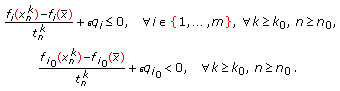 (4.31)
 and
and  such that
  . Hence, there exists
  such that
  , for all
  . It is easy to see that, if we take an appropriate subsequences
  and
and  of
of  and
and  , respectively, then there exist an index
  ,
,  and
and  such that
Therefore,  , for all
  , and
, and  , which is a contradiction to the assumption. This completes the proof.
Remark 4.18.
The following necessary conditions for  -local weakly (efficient) solutions may not be true.

See the following example.
Example 4.19.
Let  ,
,


, ,
,  ,
,  . Consider the following problem:

It is easy to see that  is an
is an  -efficient solution of (MP), but,
  . In fact,


, for all  . It is obvious that
  . On the other hand,
  . Hence,
  .
.
References
Miettinen K, Mäkelä MM: On cone characterizations of weak, proper and Pareto optimality in multiobjective optimization. Mathematical Methods of Operations Research 2001, 53(2):233–245. 10.1007/s001860000109
Huang LG, Liu SY: Cone characterizations of Pareto, weak and proper efficient points. Journal of Systems Science and Mathematical Sciences 2003, 23(4):452–460.
Engau A, Wiecek MM: Cone characterizations of approximate solutions in real vector optimization. Journal of Optimization Theory and Applications 2007, 134(3):499–513. 10.1007/s10957-007-9235-8
Aghezzaf B, Hachimi M: Second-order optimality conditions in multiobjective optimization problems. Journal of Optimization Theory and Applications 1999, 102(1):37–50. 10.1023/A:1021834210437
Cambini A, Martein L, Vlach M: Second-order tangent sets and optimaity conditions. Japan Advanced Studies of Science and Technology, Hokuriku, Japan; 1997.
Penot J-P: Second-order conditions for optimization problems with constraints. SIAM Journal on Control and Optimization 1999, 37(1):303–318.
Jiménez B, Novo V: Optimality conditions in differentiable vector optimization via second-order tangent sets. Applied Mathematics and Optimization 2004, 49(2):123–144.
Gutiérrez C, Jiménez B, Novo V: New second-order directional derivative and optimality conditions in scalar and vector optimization. Journal of Optimization Theory and Applications 2009, 142(1):85–106. 10.1007/s10957-009-9525-4
Bigi G: On sufficient second order optimality conditions in multiobjective optimization. Mathematical Methods of Operations Research 2006, 63(1):77–85. 10.1007/s00186-005-0013-9
Kutateladze SS: Convex -programming. Soviet Mathematics. Doklady 1979, 20: 390–1393.
Vályi I: Approximate saddle-point theorems in vector optimization. Journal of Optimization Theory and Applications 1987, 55(3):435–448. 10.1007/BF00941179
Liu J-C: -properly efficient solutions to nondifferentiable multiobjective programming problems. Applied Mathematics 1999, 12(6):109–113.
Bolintinéanu S: Vector variational principles; -efficiency and scalar stationarity. Journal of Convex Analysis 2001, 8(1):71–85.
Dutta J, Vetrivel V: On approximate minima in vector optimization. Numerical Functional Analysis and Optimization 2001, 22(7–8):845–859. 10.1081/NFA-100108312
Göpfert A, Riahi H, Tammer C, Zălinescu C: Variational Methods in Partially Ordered Spaces. Springer, New York, NY, USA; 2003:xiv+350.
Bednarczuk EM, Przybyła MJ: The vector-valued variational principle in Banach spaces ordered by cones with nonempty interiors. SIAM Journal on Optimization 2007, 18(3):907–913. 10.1137/060658989
Chen G, Huang X, Yang X: Vector Optimization. Set-Valued and Variational Analysis, Lecture Notes in Economics and Mathematical Systems. Volume 541. Springer, Berlin, Germany; 2005:x+306.
Gupta D, Mehra A: Two types of approximate saddle points. Numerical Functional Analysis and Optimization 2008, 29(5–6):532–550. 10.1080/01630560802099274
Gutiérrez C, Jiménez B, Novo V: A Set-valued ekeland's variational principle in vector optimization. SIAM Journal on Control and Optimization 2008, 47(2):883–903. 10.1137/060672868
Gutiérrez C, López R, Novo V: Generalized -quasi-solutions in multiobjective optimization problems: existence results and optimality conditions. Nonlinear Analysis: Theory, Methods & Applications 2010, 72(11):4331–4346. 10.1016/j.na.2010.02.012
White DJ: Epsilon efficiency. Journal of Optimization Theory and Applications 1986, 49(2):319–337. 10.1007/BF00940762
Helbig S: One new concept for -efficency. talk at Optimization Days, Montreal, Canada, 1992
Tanaka T: A new approach to approximation of solutions in vector optimization problems. In Proceedings of APORS. Volume 1995. Edited by: Fushimi M, Tone K. World Scientific, Singapore; 1994:497–504.
Sawaragi Y, Nakayama H, Tanino T: Theory of Multiobjective Optimization, Mathematics in Science and Engineering. Volume 176. Academic Press, Orlando, Fla, USA; 1985:xiii+296.
Rong WD, Ma Y: -properly efficient solution of vector optimization problems with set-valued maps. OR Transaction 2000, 4: 21–32.
Borwein J: Proper efficient points for maximizations with respect to cones. SIAM Journal on Control and Optimization 1977, 15(1):57–63. 10.1137/0315004
Huang LR: Separate necessary and sufficient conditions for the local minimum of a function. Journal of Optimization Theory and Applications 2005, 125(1):241–246. 10.1007/s10957-004-1726-2
Rudin W: Functional Analysis, McGraw-Hill Series in Higher Mathematics. McGraw-Hill, New York, NY, USA; 1973:xiii+397.
Acknowledgments
This work was partially supported by the National Science Foundation of China (no. 10771228 and 10831009), the Research Committee of The Hong Kong Polytechnic University, the Doctoral Foundation of Chongqing Normal University (no.10XLB015) and the Natural Science Foundation project of CQ CSTC (no. CSTC. 2010BB2090).
Author information
Authors and Affiliations
Corresponding author
Rights and permissions
Open Access This article is distributed under the terms of the Creative Commons Attribution 2.0 International License (https://creativecommons.org/licenses/by/2.0), which permits unrestricted use, distribution, and reproduction in any medium, provided the original work is properly cited.
About this article
Cite this article
Gao, Y., Yang, X. & Lee, H. Optimality Conditions for Approximate Solutions in Multiobjective Optimization Problems. J Inequal Appl 2010, 620928 (2010). https://doi.org/10.1155/2010/620928
Received:
Accepted:
Published:
DOI: https://doi.org/10.1155/2010/620928