Oscillations of Second-Order Neutral Impulsive Differential Equations

Abstract

Necessary and sufficient conditions are established for oscillation of second-order neutral impulsive differential equation , , where the coefficients ; , and .

1. Introduction

Oscillation theory is one of the directions which initiated the investigations of the qualitative properties of differential equations. This theory started with the classical works of Sturm and Kneser, and still attracts the attention of many mathematicians as much for the interesting results obtained as for their various applications.

In 1989 the paper of Gopalsamy and Zhang [1] was published, where the first investigation on oscillatory properties of impulsive differential equations was carried out.

The monograph [2] is the first book to present systematically the results known up to 1998, and to demonstrate how well-know mathematical techniques and methods, after suitable modification, can be applied in proving oscillatory theorems for impulsive differential equations.

Recently, the oscillatory theory of differential equations has been the subject of intensive research [3–8]. In particular, many remarkable results for the oscillatory properties of various classes of impulsive differential equations can be found in the literature [2, 9–11].

The notion of characteristic system was first introduced by Bainov and Simeonov [2]; it can be used in obtaining of various necessary and sufficient conditions for oscillation of constant coefficients linear impulsive differential equations of first order with one or several deviating arguments.

As we know, on the case when we investigate constant coefficients linear neutral differential equations without impulse, it is very significant to obtain necessary and sufficient conditions for the oscillation corresponding to their characteristic equations; some necessary and sufficient conditions (in terms of the characteristic equation) for the oscillation of all solutions of first-or second-order neutral differential equations were established in [12–20]. However, the oscillation theory of the second order impulsive differential equations is not yet perfect compared to the second order differential equations with deviating argument (see [2]). For example, due to some obstacles of theoretical and technical character in handling with constant coefficients linear impulsive differential equations of second or higher order, there are no results which studied the necessary and sufficient conditions in monograph [2]. How to establish the necessary and sufficient conditions for second order constant coefficients linear impulsive differential equations corresponding to their characteristic systems? This is also an important open problem (see monograph [2]). In this paper, we study and solve this problem for a class of linear impulsive differential equations of second order with advanced argument.

We shall restrict ourselves to the studying of impulsive differential equations for which the impulse effects take part at fixed moments . Considering the second order neutral impulsive differential equations with constant coefficients

(1.1)

where

(1.2)

Throughout this paper, we assume that the sequence of the moments of impulse effects has the following properties (H):

and

Here considering -periodic and -periodic equation with , we suppose that the sequence satisfies the following conditions.

There exist nonnegative integers and such that

(1.3)

This condition is equivalent to the next one.

There exist nonnegative integers and such that

(1.4)

Here denotes the number of the points , lying in the interval .

As customary, a solution of (1.1) is said to be oscillatory if it has arbitrarily large zeros. Otherwise the solution is called nonoscillatory. As usual, we use the term "finally" to mean "for sufficiently large ". For other related notions, see monographs [2, 9–11] for details.

We clearly see that (1.1) is an equation without impulse and together with if in (H1.2) or (H1.3). In this case, (1.1) reduces to

(1.5)

2. Asymptotic Behavior of the Solutions

In the sequence, we assume that conditions (H1.1)–(H1.3) hold, and

(2.1)

Lemma 2.1.

Suppose that is defined by (2.1). If (1.1) has a finally positive solution , then

(a) is also a solution of (1.1), that is,

(2.2)

(b)

(2.3)

or

(2.4)

• (c) If (2.3) holds, then .

• (d) If is a solution of (1.1), then

(2.5)

is also a solution of (1.1).

Proof.

• (a) It follows from condition (H1.2) that if is a moment of impulse effect, then is also a such moment. Thus, is also a solution of (1.1) since (1.1) is a linear one with constant coefficients. Therefore, is a solution of (1.1) which follows from the linear combination of solutions.

• (b) We clearly see that

(2.6)

which imply that is strictly increasing and so either

(2.7)

or

(2.8)

We clearly see that (2.7) implies inequality (2.4). Now, we assume that inequality (2.8) holds. We first prove that .

In fact, integrating (2.6) from to and letting we get

(2.9)

hence

(2.10)

which implies that is integrable in ,

(2.11)

Then from (2.1) we get

(2.12)

and so . (Otherwise, by L'Hospital's rule, we have when then ). Thus increases to zero, which implies that eventually

(2.13)

Then decreases and in view of , we have

(2.14)

hence

(2.15)

• (c) For the sake of contradiction, assume that (2.3) holds and . From parts (a) and (b), we know that 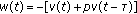is also a positive solution of (1.1), therefore,

(2.16)

which implies that

(2.17)

this contradicts with the fact that is a decreasing function.

• (d) Let be a solution of (1.1), and

(2.18)

We prove that is also a solution of (1.1).

Clearly, satisfies

(2.19)

Since is a solution of (1.1), so

(2.20)

That is,

(2.21)

which implies that is also a solution of (1.1).

Let and be the set of all functions of the form

(2.22)

where is a solution of (1.1) which satisfies (2.3) and (2.4), respectively. In view of Lemma 2.1, either or is nonempty. Also, an argument similar to that of Lemma 2.1 shows that each function is a solution of (1.1), and satisfies

(2.23)

Also, there is a solution of (1.1) which satisfies (2.3) if or (2.4) if such that

(2.24)

Clearly, every function satisfies

(2.25)

while every function satisfies

(2.26)

Furthermore,

(2.27)

Finally, (, resp.) and (, resp.).

3. Oscillation of the Unbounded Solutions

First, we will assume that (i.e.,

The present section is devoted to the characterizing of the oscillatory properties of solutions of the periodic neutral impulsive differential equation (1.1).

We are looking for a positive solution of (1.1) having the form

(3.1)

where are constants.

Substituting (3.1) in (1.1), and from condition (H1.3), we obtain the characteristic system of (1.1) as follows:

(3.2)

As , the characteristic system is equivalent to

(3.3)

Equation (3.3) is called a characteristic equation, corresponding to the (1.1).

Theorem 3.1.

If the conditions (H1.1)–(H1.3) hold, then the following assertions are equivalent.

(a)Each unbounded regular solution of (1.1) is oscillatory.

(b)The characteristic equation (3.3) has no positive real roots.

The proof of (a) (b) is obvious. In fact, if the characteristic equation (3.3) has a real root , then we clearly see that and therefore the function

(3.4)

is an unbounded positive solution of (1.1).

The proof of (b) (a) is quite complicated and will be accomplished by establishing a series of lemmas.

We assume that (3.3) has no positive real roots and, for the sake of contradiction, we assume that (1.1) has an unbounded finally positive solution

Lemma 3.2.

If (1.1) has an eventually positive solution, then

(a)

• (b) There exists a positive constant such that

(3.5)

Proof.

• (a) Otherwise, , therefore , but is impossible because the characteristic equation has no positive real roots.

• (b) We have , and so for all .

Hence there exists a positive constant such that

(3.6)

which completes the proof of Lemma 3.2.

For each function define the set

(3.7)

Clearly, and if then . Therefore, is a nonempty subinterval of .

Lemma 3.3.

For and , we have the folloeing.

• (a) If and , then

(b) is bounded above by a positive constant , for all .

(c)If and , then

(3.8)

Proof.

• (a) From (2.23), (2.26) and the fact that and , we have

  

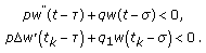  (3.9)

That is,

(3.10)

The increasing nature of and the fact that imply that

(3.11)

which shows that

(3.12)

By integrating (3.10) from to with we get

(3.13)

From the fact that and , we have

(3.14)

By integrating again from to with we get

(3.15)

from the fact that and together with , we have

(3.16)

Let then

(3.17)

That is,

(3.18)

where

Now let such that then (3.18) and the increasing nature of imply that

(3.19)

By integrating (2.24) from to with we get

(3.20)

By integrating again from to with we have

(3.21)

Let , then

(3.22)

Combining (2.24), (3.19), and (3.22), we have

(3.23)

which shows that

(3.24)

and is not in the set for all that is, is bounded above by the positive constant , for all .

• (c) Let

(3.25)

then

(3.26)

Therefore,

(3.27)

(3.28)

We clearly see that is a nondecreasing function and so if the conclusion in part (c) was false, then

(3.29)

From (3.27), (3.28), and (3.29), we know that

(3.30)

and so

(3.31)

which together with the hypothesis yield that

(3.32)

Hence

(3.33)

(3.34)

Let

(3.35)

Then by Lemma 2.1(d) and the linear combination of solutions, we know that is a solution of (1.1). From (3.29), (3.33), and (3.34), we have

(3.36)

Now using instead of in (2.1) and the hypothesis that together with a similar argument as in (2.4), we get

(3.37)

But (3.36) implies that

(3.38)

and the contradiction completes the proof of Lemma 3.3.

By integrating both sides of (2.23) from to , we get

(3.39)

That is,

(3.40)

where

(3.41)

As is a solution of (1.1) and satisfying (2.24), it follows from (3.40) that if then

(3.42)

where is the constant given by (3.41).

Lemma 3.4.

Suppose that and are the constants defined in Lemma 3.2 and Lemma 3.3, respectively. If , and

(3.43)

then

(3.44)

where

(3.45)

Proof.

Clearly is an element of . From Lemma 3.3(c), we have

(3.46)

Then from (3.45) we get

(3.47)

By integrating (3.46) from to , we obtain

(3.48)

and so

(3.49)

Let

(3.50)

then

(3.51)

By integrating it from to , we have

(3.52)

Set

(3.53)

as defined in the proof of Lemma 3.3(c).

We clearly see that is a nondecreasing function, therefore,

(3.54)

Let

(3.55)

Using (3.45), (3.47), (3.49), (3.54), the increasing nature of , and the fact that

(3.56)

we have

(3.57)

As

(3.58)

we see that for sufficiently large ,

(3.59)

and as , so

(3.60)

Then

(3.61)

Analogously,

(3.62)

Therefore, the proof of Lemma 3.4 is completed.

Now, considering the sequence of functions

(3.63)

where is the function defined by (3.45), is the number defined in Lemma 3.3(a),

(3.64)

The repeated applications of Lemma 3.4 lead to

(3.65)

Clearly

(3.66)

which contradicts with the fact proved in Lemma 3.3(b) that

(3.67)

Therefore, the proof of Theorem 3.1 is completed.

4. Oscillation of the Bounded Solutions

In Section 2, we complete the case of . Now we consider the conditions ensuring oscillation of the case of , that is, considering the conditions ensuring oscillation of the bounded solutions of (1.1). Then in view of Lemma 2.1(c), .

We are looking for a positive solution of (1.1) with the form

(4.1)

where are constants.

Substituting (4.1) in (1.1), just like in Section 2, we can obtain the characteristic equation of (1.1) as follows:

(4.2)

where

(4.3)

Theorem 4.1.

If the condition (H) holds, then the following assertions are equivalent.

• (a) Each bounded regular solution of the equation (1.5) is oscillatory.

• (b) The characteristic equation (4.2) has no real roots .

The proof of (a) (b) is obvious. In fact, if the characteristic equation (4.2) has a real root , then and , therefore the function

(4.4)

is a bounded positive solution of (1.1).

The proof of (b) (a) is quite complicated and will be accomplished by establishing a series of lemmas.

As in Section 3 we assume, without further mention, that (1.2) holds. We also assume that (4.2) has no real roots . For the sake of contradiction, we assume that (1.1) has a bounded finally positive solution .

Also like the case in Section 3, for each function define the set

(4.5)

Clearly, and if then . That is, is a nonempty subinterval of .

Lemma 4.2.

There exists a positive constant such that

(4.6)

Proof.

We clearly see that

(4.7)

and so there exists a positive constant such that

(4.8)

Lemma 4.3.

• (a) If and with , then

  

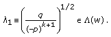  (4.9)

• (b) If and , then

(4.10)

(c) is bounded above by a positive constant for any .

Proof.

• (a) Let with

For we have

(4.11)

and so

(4.12)

That is,

(4.13)

as

(4.14)

So

(4.15)

That is,

(4.16)

• (b) Let

(4.17)

then

(4.18)

Let

(4.19)

then

(4.20)

Therefore, is a nondecreasing function.

Note that

(4.21)

We know that and so

(4.22)

• (c) Otherwise,

(4.23)

Then from part (b)

(4.24)

we know that the function is nonincreasing and

(4.25)

or

(4.26)

This contradicts with(3.54); therefore, The proof of Lemma 4.3 is completed.

Lemma 4.4.

Suppose that is a constant defined in Lemma 4.2 and . If , and

(4.27)

then

(4.28)

where

(4.29)

and

(4.30)

Proof.

Clearly, is an element of If

(4.31)

then

(4.32)

Let

(4.33)

then

(4.34)

By integrating (4.34) from to we get

(4.35)

Let then

(4.36)

Integrating (4.32) from to we get

(4.37)

That is,

(4.38)

By integrating again from to we find

(4.39)

Then from (4.35) we have

(4.40)

and

(4.41)

Using (4.29) and (4.32) together with (4.38)–(4.41), we see that

(4.42)

Therefore,

(4.43)

For and , we have . From the fact that is nonincreasing, we clearly see that . Therefore,

(4.44)

Analogously, we have

(4.45)

So

(4.46)

Therefore, the proof of Lemma 4.4 is completed.

Now, we consider the sequence of functions

(4.47)

where, is the function defined in (4.29),

(4.48)

The repeated applications of Lemma 4.4 lead to

(4.49)

Clearly,

(4.50)

which contradicts with the fact proved in Lemma 4.3(c) that is bounded above for any . Therefore, the proof of Theorem 4.1 is completed.

Remark 4.5.

Let , then (1.1) reduces to (1.5), and (3.3) and (4.2) reduce to

(4.51)

From our Theorems 3.1 and 4.1, we get the following well-known results:

Corollary 4.6.

The following assertions are equivalent.

• (a) Each unbounded regular solution of the equation (1.5) is oscillatory.

(b)The characteristic equation (4.51) has no positive real roots.

Corollary 4.7.

The following assertions are equivalent.

(a)Each bounded regular solution of the equation (1.5) is oscillatory.

(b)The characteristic equation (4.51) has no real root .

References

Gopalsamy K, Zhang BG: On delay differential equations with impulses. Journal of Mathematical Analysis and Applications 1989, 139(1):110–122. 10.1016/0022-247X(89)90232-1
Bainov D, Simeonov P: Oscillation Theory of Impulsive Differential Equations. International Publications, Orlando, Fla, USA; 1998.
Bainov DD, Mishev DP: Oscillation Theory for Neutral Differential Equations with Delay. Adam Hilger, Bristol, UK; 1991.
Győri I, Ladas G: Oscillation Theory of Delay Differential Equations. The Clarendon Press Oxford University, New York, NY, USA; 1991.
Erbe LH, Kong Q, Zhang BG: Oscillation Theory for Functional-Differential Equations. Volume 190. Marcel Dekker, New York, NY, USA; 1995.
Agarwal RP, Grace SR, O'Regan D: Oscillation Theory for Difference and Functional Differential Equations. Kluwer Academic Publishers, Dordrecht, The Netherlands; 2000.
Agarwal RP, Grace SR, O'Regan D: Oscillation Theory for Second Order Dynamic Equations. Volume 5. Taylor and Francis, London, UK; 2003.
Agarwal RP, Bohner M, Li W-T: Nonoscillation and Oscillation: Theory for Functional Differential Equations. Volume 267. Marcel Dekker, New York, NY, USA; 2004.
Lakshmikantham V, Bainov DD, Simeonov PS: Theory of Impulsive Differential Equations. Volume 6. World Scientific Publishing Company, Teaneck, NJ, USA; 1989.
Bainov D, Simeonov P: Impulsive Differential Equations: Periodic Solutions and Applications. Volume 66. Longman Scientific and Technical, Harlow, Uk; 1993.
Bainov DD, Simeonov PS: Impulsive Differential Equations. Volume 28. World Scientific Publishing Company, River Edge, NJ, USA; 1995.
Ladas G, Sficas YG, Stavroulakis IP: Necessary and sufficient conditions for oscillations of higher order delay differential equations. Transactions of the American Mathematical Society 1984, 285(1):81–90. 10.1090/S0002-9947-1984-0748831-8
Sficas YG, Stavroulakis IP: Necessary and sufficient conditions for oscillations of neutral differential equations. Journal of Mathematical Analysis and Applications 1987, 123(2):494–507. 10.1016/0022-247X(87)90326-X
Grove EA, Ladas G, Meimaridou A: A necessary and sufficient condition for the oscillation of neutral equations. Journal of Mathematical Analysis and Applications 1987, 126(2):341–354. 10.1016/0022-247X(87)90045-X
Arino O, Győri I: Necessary and sufficient condition for oscillation of a neutral differential system with several delays. Journal of Differential Equations 1989, 81(1):98–105. 10.1016/0022-0396(89)90179-4
Grammatikopoulos MK, Stavroulakis IP: Necessary and sufficient conditions for oscillation of neutral equations with deviating arguments. Journal of the London Mathematical Society. Second Series 1990, 41(2):244–260. 10.1112/jlms/s2-41.2.244
Kulenović MRS, Ladas G, Sficas YG: Oscillations of second order linear delay differential equations. Applicable Analysis 1988, 27(1–3):109–123.
Ladas G, Partheniadis EC, Sficas YG: Necessary and sufficient conditions for oscillations of second-order neutral equations. Journal of Mathematical Analysis and Applications 1989, 138(1):214–231. 10.1016/0022-247X(89)90332-6
Bilchev SJ, Grammatikopoulos MK, Stavroulakis IP: Oscillations of second-order neutral differential equations with deviating arguments. In Oscillation and Dynamics in Delay Equations (San Francisco, CA, 1991), Contemporary Mathematics. Volume 129. American Mathematical Society, Providence, RI, USA; 1992:1–21.
Wang Z: A necessary and sufficient condition for the oscillation of higher-order neutral equations. The Tohoku Mathematical Journal 1989, 41(4):575–588. 10.2748/tmj/1178227728
Acknowledgment
The authors wish to thank the anonymous referee for the very careful reading of the manuscript and fruitful comments and suggestions.
Author information
Authors and Affiliations
Corresponding author
Rights and permissions
Open Access This article is distributed under the terms of the Creative Commons Attribution 2.0 International License (https://creativecommons.org/licenses/by/2.0), which permits unrestricted use, distribution, and reproduction in any medium, provided the original work is properly cited.
About this article
Cite this article
Cheng, JF., Chu, YM. Oscillations of Second-Order Neutral Impulsive Differential Equations. J Inequal Appl 2010, 493927 (2010). https://doi.org/10.1155/2010/493927
Received:
Revised:
Accepted:
Published:
DOI: https://doi.org/10.1155/2010/493927