- Research Article
- Open access
- Published:
A Note on the Integral Inequalities with Two Dependent Limits
Journal of Inequalities and Applications volume 2010, Article number: 430512 (2010)
Abstract
The theorem on the Gronwall's type integral inequalities with two dependent limits is established. In application, the boundedness of the solutions of nonlinear differential equations is presented.
1. Introduction
Integral inequalities play a significant role in the study of qualitative properties of solutions of integral, differential and integro-differential equations (see, e.g., [1–4] and the references given therein). One of the most useful inequalities in the development of the theory of differential equations is given in the following lemma (see [5]).
Lemma 1.1.
Let  and
and  be real-valued nonnegative continuous functions for all
  . If
. If

for all  , where
  is a real constant, then

for all  .
.
Note that the generalization of this integral inequality and its discrete analogies are given in papers [5–8]. In paper [9] the following useful inequality with two dependent limits was established.
Lemma 1.2.
Let  be a real-valued nonnegative continuous function defined on
  and let
  and
and  be nonnegative constants. Then the inequality

implies that

The theory of integral inequalities with several dependent limits and its applications to differential equations has been investigated in [10–14].
The present study involves some Gronwall's type integral inequalities with two dependent limits. Section 2 includes some new integral inequalities with two dependent limits and relevant proofs. Subsequently, Section 3 includes an application on the boundedness of the solutions of nonlinear differential equations.
2. A Main Statement
Our main statement is given by the following theorem.
Theorem 2.1.
Let  ,
,  ,
,  ,
,  ,
,  , and
, and  be real-valued nonnegative continuous functions defined on
  .
.
-
(i)
Let
 be a nonnegative constant. If
 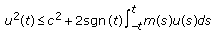 (2.1)
(2.1)
 be a nonnegative constant. If
for  then
then

for all 
-
(ii)
Let
 be a real constant. If
  (2.3)
(2.3)
 be a real constant. If
for  then
then

for all 
-
(iii)
Let
 be a real-valued positive continuous and nondecreasing function defined on
  and
and  be a real constant. If
 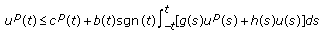 (2.5)
(2.5)
 be a real-valued positive continuous and nondecreasing function defined on
  and
and  be a real constant. If
for  then
then

for all 
-
(iv)
Let
 and its partial derivative
  be real-valued nonnegative continuous functions on
  and let
 be even function in
  If
If  (2.7)
(2.7)
 and its partial derivative
  be real-valued nonnegative continuous functions on
  and let
 be even function in
  If
If 
for  then
then

for all  . Here

where


Proof.
-
(i)
Define a function
 by
by  (2.12)
 by
by 
Note that  is a nonnegative function and
  Then (2.1) can be rewritten as

It is easy to see that  is an even function.
First, let  ; then (2.12) can be rewritten as

Differentiating (2.14) and using (2.13), we get

Dividing both sides of (2.15) by  , we get

Integrating the last inequality from  to
to  , we get

Second, let  . Then, (2.12) can be written as

Differentiating (2.18) and using (2.13), we get

Dividing both sides of (2.19) by  , we get

Integrating (2.20) from  to 0, we get

Finally, using (2.17) and (2.21), we obtain

The inequality (2.2) follows from (2.13) and (2.22).
-
(ii)
Define a function
 by
by 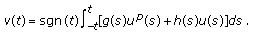 (2.23)
 by
by 
It is evident that  is an even and nonnegative function. We have that

Using Young's inequality (see, e.g., [2]), we obtain that

Let  . Then

Differentiating (2.26), we get

Using (2.24) and (2.25), we get

Denoting

we get

From that it follows that

for any  Integrating the last inequality from
  to
to  and using
  , we get

It is easy to see that

Then

Since  , we have that

Applying (2.24), we obtain

From (2.36), and (2.29) it follows (2.4) for  Let
Let  ; then

Using (2.24) and (2.25), we get

From that it follows that

for any  Integrating the last inequality from
  to
to  and using
  , we get

It is easy to see that

Then

Since  , we have that

Applying (2.43) and (2.24), we obtain (2.36) for  Then from (2.36) and (2.29), (2.4) follows for
-
(iii)
Since
 is a positive, continuous, and nondecreasing function for
  , we have that
 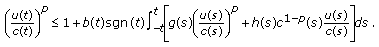 (2.44)
 is a positive, continuous, and nondecreasing function for
  , we have that
Now the application of the inequality proven in (ii) yields the desired result in (2.6).
-
(iv)
We define a function
 by
by  (2.45)
 by
by 
Evidently, the function  is a nonnegative, monotonic, and nondecreasing in
  and
and  We have that

Let  . Then

Differentiating (2.47), we get

Using (2.46) and Young's inequality, we obtain that

Using (2.29), we get

Applying the differential inequality, we get

Since  , we have that

Using (2.33), we get

Since  , we have that

Using (2.9) and (2.11), we get

Let  . Then

Differentiating (2.56), we get

Using (2.46) and Young's inequality, we obtain that

Using (2.29), we get

Applying the differential inequality, we get

Since  , we have that

Using (2.41), we get

Since  , we have that

Using (2.9) and (2.10), we get

The inequality (2.8) follows from (2.29), (2.55), and (2.64). Theorem 2.1 is proved.
3. An Application
In this section, we indicate an application of Theorem 2.1 (part (ii)) to obtain the explicit bound on the solution of the following boundary value problem for one dimensional partial differential equations:

where  is a fixed real number and
  . Let
. Let  ,
,  ,
,  ,
,  ,
,  ,
,  be smooth functions and problem (3.1) has a unique smooth solution
  Assume that

for all  Here
Here and
and are real-valued nonnegative continuous functions defined on
  .
.
This allows us to reduce the nonlocal boundary-value (3.1) to the initial-value problem

in a Hilbert space  with a self-adjoint positive definite operator
  defined by the formula
  with the domain

 (see, e.g., [15, 16]).
Let us give a corollary of Theorem 2.1.
Theorem 3.1.
The solution of problem (3.1) satisfies the estimates

for all  Here
Here 
Proof.
It is known thatthe formula (see, e.g., [15, 16])

gives a solution of problem ( 3.3 ). Here

Applying the triangle inequality, condition (3.2), formula (3.5), and estimates (see, e.g., [17])

we get

Since

we have that

Denote that  Then
Then

for  Applying the integral inequality (2.4), we get

We have that

Therefore, the inequality (3.4) follows from the last inequality. Theorem 3.1 is proved.
References
Agarwal RP: Difference Equations and Inequalities: Theory, Methods and Applications, Monographs and Textbooks in Pure and Applied Mathematics. Volume 155. Marcel Dekker, New York, NY, USA; 1992:xiv+777.
Beckenbach EF, Bellman R: Inequalities. Springer, New York, NY, USA; 1965:xi+198.
Mitrinović DS: Analytic Inequalities. Springer, New York, NY, USA; 1970:xii+400.
Gronwall TH: Note on the derivatives with respect to a parameter of the solutions of a system of differential equations. Annals of Mathematics II 1919, 20(4):292–296.
Pachpatte BG: Some new finite difference inequalities. Computers & Mathematics with Applications 1994, 28(1–3):227–241.
Kurpınar E: On inequalities in the theory of differential equations and their discrete analogues. Pan-American Mathematical Journal 1999, 9(4):55–67.
Pachpatte BG: On the discrete generalizations of Gronwall's inequality. Journal of Indian Mathematical Society 1973, 37: 147–156.
Pachpatte BG: Inequalities for Differential and Integral Equations, Mathematics in Science and Engineering. Volume 197. Academic Press, New York, NY, USA; 1998:x+611.
Mamedov YDj, Ashirov S: A Volterra type integral equation. Ukrainian Mathematical Journal 1988, 40(4):510–515.
Ashyraliyev M: Generalizations of Gronwall's integral inequality and their discrete analogies. Report September 2005., (MAS-EO520):
Ashyraliyev M: Integral inequalities with four variable limits. In Modeling the Processes in Exploration of Gas Deposits and Applied Problems of Theoretical Gas Hydrodynamics. Ylym, Ashgabat, Turkmenistan; 1998:170–184.
Ashyraliyev M: A note on the stability of the integral-differential equation of the hyperbolic type in a Hilbert space. Numerical Functional Analysis and Optimization 2008, 29(7–8):750–769. 10.1080/01630560802292069
Ashirov S, Kurbanmamedov N: Investigation of the solution of a class of integral equations of Volterra type. Izvestiya Vysshikh Uchebnykh Zavedeniĭ. Matematika 1987, 9: 3–9.
Corduneanu A: A note on the Gronwall inequality in two independent variables. Journal of Integral Equations 1982, 4(3):271–276.
Fattorini HO: Second Order Linear Differential Equations in Banach Spaces, Notas de Matematica, North-Holland Mathematics Studies. Volume 108. North-Holland, Amsterdam, The Netherlands; 1985:xiii+314.
Piskarev S, Shaw S-Y: On certain operator families related to cosine operator functions. Taiwanese Journal of Mathematics 1997, 1(4):3585–3592.
Ashyralyev A, Aggez N: A note on the difference schemes of the nonlocal boundary value problems for hyperbolic equations. Numerical Functional Analysis and Optimization 2004, 25(5–6):439–462. 10.1081/NFA-200041711
Acknowledgments
The authors thank professor O. Celebi (Turkey), professor R. P. Agarwal (USA), and anonymous reviewers for their valuable comments.
Author information
Authors and Affiliations
Corresponding author
Rights and permissions
Open Access This article is distributed under the terms of the Creative Commons Attribution 2.0 International License ( https://creativecommons.org/licenses/by/2.0 ), which permits unrestricted use, distribution, and reproduction in any medium, provided the original work is properly cited.
About this article
Cite this article
Ashyralyev, A., Misirli, E. & Mogol, O. A Note on the Integral Inequalities with Two Dependent Limits. J Inequal Appl 2010, 430512 (2010). https://doi.org/10.1155/2010/430512
Received:
Revised:
Accepted:
Published:
DOI: https://doi.org/10.1155/2010/430512