A New Hilbert-Type Linear Operator with a Composite Kernel and Its Applications

Abstract

A new Hilbert-type linear operator with a composite kernel function is built. As the applications, two new more accurate operator inequalities and their equivalent forms are deduced. The constant factors in these inequalities are proved to be the best possible.

1. Introduction

In 1908, Weyl [1] published the well-known Hilbert's inequality as follows:

if , are real sequences, and , then

(1.1)

where the constant factor is the best possible.

Under the same conditions, there are the classical inequalities [2]

(1.2)

(1.3)

where the constant factors and are the best possible also. Expression (1.2) is called a more accurate form of(1.1). Some more accurate inequalities were considered by [3–5]. In 2009, Zhong [5] gave a more accurate form of (1.3).

Set , as two pairs of conjugate exponents, and , , , and , , such that and , then it has

(1.4)

Letting , , , , , and , the expression (1.4) can be rewritten as

(1.5)

where is a linear operator, . is the norm of the sequence with a weight function . is a formal inner product of the sequences and .

By setting two monotonic increasing functions and , a new Hilbert-type inequality, which is with a composite kernel function , and its equivalent are built in this paper. As the applications, two new more accurate Hilbert-type inequalities incorporating the linear operator and the norm are deduced.

Firstly, the improved Euler-Maclaurin's summation formula [6] is introduced.

Set . If , (), then it has

(1.6)

2. Lemmas

Lemma 2.1.

Set as a pair of conjugate exponents, , , , and define

(2.1)

(2.2)

(2.3)

(2.4)

(2.5)

Then, it has the following.

(1)The functions , satisfy the conditions of (1.6). It means that

(2.6)

(2) 

(2.7)

(3) 

(2.8)

Proof.

• (1) For , , , , and , set

  

  (2.9)

It has

(2.10)

when . It is easy to find that

(2.11)

Similarly, it can be shown that , (, ). These tell us that (2.6) holds and the functions , satisfy the conditions of (1.6).

• (2) Set . With the partial integration, it has

  

  (2.12)

By (2.1), it has

(2.13)

(2.14)

In view of (2.12)~(2.14), it has

(2.15)

As , , and , it has

(2.16)

It means that . Similarly, it can be shown that . The expression (2.7) holds.

• (3) By (2.5), (2.12), (2.13), and , , it has

  

  (2.17)

The expression (2.8) holds, and Lemma 2.1 is proved.

Lemma 2.2.

Set as a pair of conjugate exponents, , , and , and define

(2.18)

Then, it has

(1)The functions , satisfy the conditions of (1.6). It means that

(2.19)

(2) 

(2.20)

(3) 

(2.21)

Proof.

• (1) Letting , , it can be proved that satisfy (2.19) as in [5]. Similarly, it can be shown that satisfy (2.19) also.

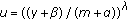
• (2) Setting , by ,, and , it has

  

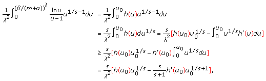  (2.22)

(2.23)

(2.24)

With (2.22)~(2.24), it has

(2.25)

By , , and , , , it has

(2.26)

So holds. Similarly, it can be shown that .

• (3) In view of (2.22), (2.23), by , , it has

  

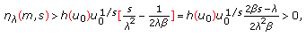  (2.27)

and by , so there exists a constant , such that (). Then it has

(2.28)

It means that (2.21) holds. The proof for Lemma 2.2 is finished.

3. Main Results

Set , ,,, and as two pairs of conjugate exponents. is a measurable kernel function. Both and are strictly monotonic increasing differentiable functions in such that ,. Give some notations as follows:

• (1)
  

  (3.1)

(2)set

(3.2)

and call a real space of sequences, where

(3.3)

is called the norm of the sequence with a weight function. Similarly, the real spaces of sequences, and the norm can be defined as well,

• (3) define a Hilbert-type linear operator, for all ,

(3.4)

• (4) for all , , define the formal inner product ofand as

(3.5)

define two weight coefficients and as

(3.6)

Then it has some results in the following theorems.

Theorem 3.1.

Suppose that , , and . If there exists a positive number , such that

(3.7)

(3.8)

then for all and , it has the following:

(1) 

(3.9)

It means that ,

(2) is a bounded linear operator and

(3.10)

where , are defined by (3.4), is defined as (3.3).

Proof.

By using Hölder's inequality [7] and (3.6), (3.7), it has and

(3.11)

And by , it follows that

(3.12)

This means that , , and . is a bounded linear operator.

If there exists a constant , such that , then for , setting , , it has , , and

(3.13)

But on the other side, by (3.8), it has

(3.14)

By the strictly monotonic increase of and , , there exists such that for all . So it has

(3.15)

The series is uniformly convergent for , so it has

(3.16)

and for , there exists , when , it has

(3.17)

By (3.14) and (3.8), when , it has

(3.18)

In view of (3.13) and (3.18), letting , it has . This means that ; that is, . Theorem 3.1 is proved.

Theorem 3.2.

Suppose that and are two pairs of conjugate exponents, , , . Let

(3.19)

Here, , satisfy the conditions as in Theorem 3.1. Set

(3.20)

(3.21)

(3.22)

If (a) is a homogeneous measurable kernel function of "'' degree in , such that

(3.23)

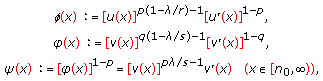
• (b) functions , satisfy the conditions of (1.6); that is,

  

  (3.24)

• (c) there exists , such that

  

  (3.25)

then it has

(1)if , , and , , then

(3.26)

(2)if and , then

(3.27)

where inequality (3.27) is equivalent to (3.26) and the constant factor is the best possible.

Proof.

By (3.24), (1.6), it has

(3.28)

(3.29)

Letting and in the integral of (3.28) and (3.29), respectively, by (3.23), it has

(3.30)

(3.31)

(where, letting , it has ). In view of (3.28), (3.30), (3.20), (3.22), and with (3.25), it has

(3.32)

Similarly, with (3.29), (3.31), (3.21), and (3.25), it has

(3.33)

also. By Theorem 3.1, it has

(3.34)

and (3.27) holds. In view of

(3.35)

(3.26) holds also.

If (3.26) holds, from (3.26) and , there exists , such that and when . For , it has

(3.36)

By and , it follows that

(3.37)

Letting in (3.37), it has , and it means that and . Therefore, the inequality (3.36) keeps the form of the strict inequality when . In view of , inequality (3.27) holds and (3.27) is equivalent to (3.26). By , it is obvious that the constant factor is the best possible. This completes the proof of Theorem 3.2.

4. Applications

Example 4.1.

Set , be two pairs of conjugate exponents and , , , . Then it has the following.

(1)If , and , then

(4.1)

(2)If , then

(4.2)

where the constant factors and are both the best possible. Inequality (4.2) is equivalent to (4.1).

Proof.

Setting , , it is a homogeneous measurable kernel function of "'' degree. Letting , it has

(4.3)

Setting , , then both and are strictly monotonic increasing differentiable functions in and satisfy

(4.4)

for . As , , , and , letting

(4.5)

with (2.1)~(2.8), it has

(4.6)

When and ; that is, , and , , by Theorem 3.2, inequality (4.1) holds, so does (4.2). And (4.2) is equivalent to (4.1), and the constant factors and are both the best possible.

Example 4.2.

Set , be two pairs of conjugate exponents and , , , . Then it has the following.

(1)If and , then

(4.7)

(2)If , then

(4.8)

where inequality (4.8) is equivalent to (4.7) and the constant factors and are both the best possible.

Proof.

Setting , it is a homogeneous measurable kernel function of "'' degree. Letting , it has [2]

(4.9)

Setting , , then both and are strictly monotonic increasing differentiable functions in and satisfy

(4.10)

for . As , , , and , letting

(4.11)

with (2.18)~(2.21), it has

(4.12)

When and ; that is, , and , , by Theorem 3.2, inequality (4.7) holds, so does (4.8). And (4.8) is equivalent to (4.7), and the constant factors and are both the best possible.

Remark 4.3.

It can be proved similarly that, if the conditions "" in Lemma 2.1 and "" in Lemma 2.2 are changed into "" and "", respectively, Lemmas 2.1 and 2.2 are also valid. So the conditions "" in Example 4.1 and "" in Example 4.2 can be replaced by ", " and ", ", respectively.

References

Weyl H: Singulare Integralgleichungen mit besonderer Beriicksichtigung des Fourierschen Integraltheorems, Inaugeral dissertation. University of Göttingen, Göttingen, Germany; 1908.
Hardy G, Littiewood J, Polya G: Inequalities. Cambridge University Press, Cambridge, UK; 1934.
Yang BC: On a more accurate Hardy-Hilbert-type inequality and its applications. Acta Mathematica Sinica 2006, 49(2):363–368.
Yang B: On a more accurate Hilbert's type inequality. International Mathematical Forum 2007, 2(37–40):1831–1837.
Zhong W: A Hilbert-type linear operator with the norm and its applications. Journal of Inequalities and Applications 2009, 2009:-18.
Yang B: The Norm of Operator and Hilbert-Type Inequalities. Science Press, Beijing, China; 2009.
Kuang J: Applied Inequalities. Shangdong Science and Technology Press, Jinan, China; 2004.
Acknowledgment
This paper is supported by the National Natural Science Foundation of China (no. 10871073). The author would like to thank the anonymous referee for his or her suggestions and corrections.
Author information
Authors and Affiliations
Corresponding author
Rights and permissions
Open Access This article is distributed under the terms of the Creative Commons Attribution 2.0 International License (https://creativecommons.org/licenses/by/2.0), which permits unrestricted use, distribution, and reproduction in any medium, provided the original work is properly cited.
About this article
Cite this article
Zhong, W. A New Hilbert-Type Linear Operator with a Composite Kernel and Its Applications. J Inequal Appl 2010, 393025 (2010). https://doi.org/10.1155/2010/393025
Received:
Accepted:
Published:
DOI: https://doi.org/10.1155/2010/393025