Almost Sure Central Limit Theorem for a Nonstationary Gaussian Sequence

Abstract

Let be a standardized non-stationary Gaussian sequence, and let denote , . Under some additional condition, let the constants satisfy as for some and , for some , then, we have almost surely for any , where is the indicator function of the event and stands for the standard normal distribution function.

1. Introduction

When is a sequence of independent and identically distributed (i.i.d.) random variables and for . If , the so-called almost sure central limit theorem (ASCLT) has the simplest form as follows:

(1.1)

almost surely for all , where is the indicator function of the event and stands for the standard normal distribution function. This result was first proved independently by Brosamler [1] and Schatte [2] under a stronger moment condition; since then, this type of almost sure version was extended to different directions. For example, Fahrner and Stadtmüller [3] and Cheng et al. [4] extended this almost sure convergence for partial sums to the case of maxima of i.i.d. random variables. Under some natural conditions, they proved as follows:

(1.2)

for all , where and satisfy

(1.3)

for any continuity point of .

In a related work, Csáki and Gonchigdanzan [5] investigated the validity of (1.2) for maxima of stationary Gaussian sequences under some mild condition whereas Chen and Lin [6] extended it to non-stationary Gaussian sequences. Recently, Dudziński [7] obtained two-dimensional version for a standardized stationary Gaussian sequence. In this paper, inspired by the above results, we further study ASCLT in the joint version for a non-stationary Gaussian sequence.

2. Main Result

Throughout this paper, let be a non-stationary standardized normal sequence, and . Here and stand for and , respectively. is the standard normal distribution function, and is its density function; will denote a positive constant although its value may change from one appearance to the next. Now, we state our main result as follows.

Theorem 2.1.

Let be a sequence of non-stationary standardized Gaussian variables with covariance matrix such that for , where for all and . If the constants satisfy as for some and , for some , then

(2.1)

almost surely for any .

Remark 2.2.

The condition is inspired by (a1) in Dudziński [8], which is much more weaker.

3. Proof

First, we introduce the following lemmas which will be used to prove our main result.

Lemma 3.1.

Under the assumptions of Theorem 2.1, one has

(3.1)

Proof.

This lemma comes from Chen and Lin [6].

The following lemma is Theorem 2.1 and Corollary in Li and Shao [9].

Lemma 3.2.

• (1) Let and be sequences of standard Gaussian variables with covariance matrices and , respectively. Put 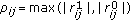. Then one has

  

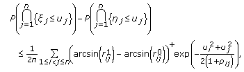  (3.2)

for any real numbers , .

• (2) Let be standard Gaussian variables with . Then

  

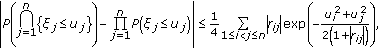  (3.3)

for any real numbers , .

Lemma 3.3.

Let be a sequence of standard Gaussian variables and satisfy the conditions of Theorem 2.1, then for , one has

(3.4)

for any .

Proof.

By the conditions of Theorem 2.1, we have

(3.5)

then, for , by , it follows that

(3.6)

Then, there exist numbers , , such that, for any , we have

(3.7)

We can write that

(3.8)

where is a random variable, which has the same distribution as , but it is independent of For apply Lemma 3.2 (1) with Then for and for . Thus, we have (for )

(3.9)

Since (3.5), (3.7) hold, we obtain

(3.10)

Now define by . By the well-known fact

(3.11)

it is easy to see that

(3.12)

Thus, according to the assumption , we have for some . Hence

(3.13)

Now, we are in a position to estimate . Observe that

(3.14)

For , it follows that

(3.15)

By Lemma 3.2 (2), we have

(3.16)

Thus by Lemma 3.1 we obtain the desired result.

Lemma 3.4.

Let be a sequence of standard Gaussian variables satisfying the conditions of Theorem 2.1, then for , any , one has

(3.17)

Proof.

Apply Lemma 3.2 (1) with (, , , , , ), (), where has the same distribution as , but it is independent of . Then,

(3.18)

Thus, combined with (3.5), (3.7), it follows that

(3.19)

Using Lemma 3.1, we have

(3.20)

By the similar technique that was applied to prove (3.10), we obtain

(3.21)

For , by , and (3.12), we have

(3.22)

As to , by (3.5) and (3.6), we have

(3.23)

Thus the proof of this lemma is completed.

Proof of Theorem 2.1.

First, by assumptions and Theorem in Leadbetter et al. [10], we have

(3.24)

Let denote a random variable which has the same distribution as , but it is independent of then by (3.10), we derive

(3.25)

Thus, by the standard normal property of , we have

(3.26)

Hence, to complete the proof, it is sufficient to show

(3.27)

In order to show this, by Lemma 3.1 in Csáki and Gonchigdanzan [5], we only need to prove

(3.28)

for and any . Let . Then

(3.29)

Since , it follows that

(3.30)

Now, we turn to estimate . Observe that for

(3.31)

By Lemma 3.3, we have

(3.32)

Using Lemma 3.4, it follows that

(3.33)

Hence for , we have

(3.34)

Consequently

(3.35)

Thus, we complete the proof of (3.28) by (3.30) and (3.35). Further, our main result is proved.

References

Brosamler GA: An almost everywhere central limit theorem. Mathematical Proceedings of the Cambridge Philosophical Society 1988, 104(3):561–574. 10.1017/S0305004100065750
Schatte P: On strong versions of the central limit theorem. Mathematische Nachrichten 1988, 137: 249–256. 10.1002/mana.19881370117
Fahrner I, Stadtmüller U: On almost sure max-limit theorems. Statistics & Probability Letters 1998, 37(3):229–236. 10.1016/S0167-7152(97)00121-1
Cheng S, Peng L, Qi Y: Almost sure convergence in extreme value theory. Mathematische Nachrichten 1998, 190: 43–50. 10.1002/mana.19981900104
Csáki E, Gonchigdanzan K: Almost sure limit theorems for the maximum of stationary Gaussian sequences. Statistics & Probability Letters 2002, 58(2):195–203. 10.1016/S0167-7152(02)00128-1
Chen S, Lin Z: Almost sure max-limits for nonstationary Gaussian sequence. Statistics & Probability Letters 2006, 76(11):1175–1184. 10.1016/j.spl.2005.12.018
Dudziński M: The almost sure central limit theorems in the joint version for the maxima and sums of certain stationary Gaussian sequences. Statistics & Probability Letters 2008, 78(4):347–357. 10.1016/j.spl.2007.07.007
Dudziński M: An almost sure limit theorem for the maxima and sums of stationary Gaussian sequences. Probability and Mathematical Statistics 2003, 23(1):139–152.
Li WV, Shao Q: A normal comparison inequality and its applications. Probability Theory and Related Fields 2002, 122(4):494–508. 10.1007/s004400100176
Leadbetter MR, Lindgren G, Rootzén H: Extremes and Related Properties of Random Sequences and Processes, Springer Series in Statistics. Springer, New York, NY, USA; 1983:xii+336.
Acknowledgments
The author thanks the referees for pointing out some errors in a previous version, as well as for several comments that have led to improvements in this paper. The authors would like to thank Professor Zuoxiang Peng of Southwest University in China for his help. The paper has been supported by the young excellent talent foundation of Huaiyin Normal University.
Author information
Authors and Affiliations
Corresponding author
Rights and permissions
Open Access This article is distributed under the terms of the Creative Commons Attribution 2.0 International License (https://creativecommons.org/licenses/by/2.0), which permits unrestricted use, distribution, and reproduction in any medium, provided the original work is properly cited.
About this article
Cite this article
Zang, Qp. Almost Sure Central Limit Theorem for a Nonstationary Gaussian Sequence. J Inequal Appl 2010, 130915 (2010). https://doi.org/10.1155/2010/130915
Received:
Revised:
Accepted:
Published:
DOI: https://doi.org/10.1155/2010/130915