New Trace Bounds for the Product of Two Matrices and Their Applications in the Algebraic Riccati Equation

Abstract

By using singular value decomposition and majorization inequalities, we propose new inequalities for the trace of the product of two arbitrary real square matrices. These bounds improve and extend the recent results. Further, we give their application in the algebraic Riccati equation. Finally, numerical examples have illustrated that our results are effective and superior.

1. Introduction

In the analysis and design of controllers and filters for linear dynamical systems, the Riccati equation is of great importance in both theory and practice (see [1–5]). Consider the following linear system (see [4]):

(1.1)

with the cost

(1.2)

Moreover, the optimal control rate and the optimal cost of (1.1) and (1.2) are

(1.3)

where is the initial state of the systems (1.1) and (1.2), is the positive definite solution of the following algebraic Riccati equation (ARE):

(1.4)

with and are symmetric positive definite matrices. To guarantee the existence of the positive definite solution to (1.4), we shall make the following assumptions: the pair () is stabilizable, and the pair () is observable.

In practice, it is hard to solve the (ARE), and there is no general method unless the system matrices are special and there are some methods and algorithms to solve (1.4), however, the solution can be time-consuming and computationally difficult, particularly as the dimensions of the system matrices increase. Thus, a number of works have been presented by researchers to evaluate the bounds and trace bounds for the solution of the (ARE) [6–12]. In addition, from [2, 6], we know that an interpretation of is that is the average value of the optimal cost as varies over the surface of a unit sphere. Therefore, consider its applications, it is important to discuss trace bounds for the product of two matrices. Most available results are based on the assumption that at least one matrix is symmetric [7, 8, 11, 12]. However, it is important and difficult to get an estimate of the trace bounds when any matrix in the product is nonsymmetric in theory and practice. There are some results in [13–15].

In this paper, we propose new trace bounds for the product of two general matrices. The new trace bounds improve the recent results. Then, for their application in the algebraic Riccati equation, we get some upper and lower bounds.

In the following, let denote the set of real matrices. Let be a real -element array which is reordered, and its elements are arranged in nonincreasing order. That is, . Let . For , let , , denote the diagonal elements, the eigenvalues, the singular values of , respectively, Let denote the trace, the transpose of , respectively. We define , The notation () is used to denote that is a symmetric positive definite (semidefinite) matrix.

Let be two real -element arrays. If they satisfy

(1.5)

then it is said that is controlled weakly by , which is signed by .

If and

(1.6)

then it is said that is controlled by , which is signed by .

Therefore, considering the application of the trace bounds, many scholars pay much attention to estimate the trace bounds for the product of two matrices.

Marshall and Olkin in [16] have showed that for any then

(1.7)

Xing et al. in [13] have observed another result. Let be arbitrary matrices with the following singular value decomposition:

(1.8)

where are orthogonal. Then

(1.9)

where is orthogonal.

Liu and He in [14] have obtained the following: let be arbitrary matrices with the following singular value decomposition:

(1.10)

where are orthogonal. Then

(1.11)

• F. Zhang and Q. Zhang in [15] have obtained the following: let be arbitrary matrices with the following singular value decomposition:

  

  (1.12)

where are orthogonal. Then

(1.13)

where is orthogonal. They show that (1.13) has improved (1.9).

2. Main Results

The following lemmas are used to prove the main results.

Lemma 2.1 (see [16, page 92, H.2.c] ).

If and , then for any real array ,

(2.1)

Lemma 2.2 (see [16, page 95, H.3.b] ).

If and , then for any real array ,

(2.2)

Remark 2.3.

Note that if , then for , . Thus from Lemma 2.2, we have

(2.3)

Lemma 2.4 (see [16, page 218, B.1] ).

Let , then

(2.4)

Lemma 2.5 (see [16, page 240, F.4.a] ).

Let , then

(2.5)

Lemma 2.6 (see [17] ).

Let . Then

(2.6)

where

(2.7)

Note that if or , obviously, (2.6) holds. If , choose , then (2.6) also holds.

Remark 2.7.

If , then we obtain Cauchy-Schwartz inequality

(2.8)

where

(2.9)

Remark 2.8.

Note that

(2.10)

Let in (2.6), then we obtain

(2.11)

Lemma 2.9.

If , , then

(2.12)

Proof.

• (1) Note that , or ,

  

  (2.13)

• (2) If , , for , choose , then and 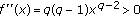. Thus, is a convex function. As and , from the property of the convex function, we have

  

  (2.14)

• (3) If , without loss of generality, we may assume . Then from (2), we have

  

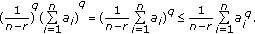  (2.15)

Since , thus

(2.16)

This completes the proof.

Theorem 2.10.

Let be arbitrary matrices with the following singular value decomposition:

(2.17)

where are orthogonal. Then

(2.18)

Proof.

By the matrix theory we have

(2.19)

Since , without loss of generality, we may assume . Next, we will prove the left-hand side of (2.18):

(2.20)

If

(2.21)

we obtain the conclusion. Now assume that there exists such that then

(2.22)

We use to denote the vector of after changing and , then

(2.23)

After limited steps, we obtain the the left-hand side of (2.18). For the right-hand side of (2.18),

(2.24)

If

(2.25)

we obtain the conclusion. Now assume that there exists such that then

(2.26)

We use to denote the vector of after changing and , then

(2.27)

After limited steps, we obtain the right-hand side of (2.18). Therefore,

(2.28)

This completes the proof.

Since applying (2.18) with in lieu of we immediately have the following corollary.

Corollary 2.11.

Let be arbitrary matrices with the following singular value decomposition:

(2.29)

where are orthogonal. Then

(2.30)

Now using (2.18) and (2.30), one finally has the following theorem.

Theorem 2.12.

Let be arbitrary matrices with the following singular value decompositions, respectively:

(2.31)

where are orthogonal. Then

(2.32)

Remark 2.13.

We point out that (2.18) improves (1.11). In fact, it is obvious that

(2.33)

This implies that (2.18) improves (1.11).

Remark 2.14.

We point out that (2.18) improves (1.13). Since for , and , from Lemmas 2.1 and 2.4, then (2.18) implies

(2.34)

In fact, for , we have

(2.35)

Then (2.34) can be rewritten as

(2.36)

This implies that (2.18) improves (1.13).

Remark 2.15.

We point out that (1.13) improves (1.7). In fact, from Lemma 2.5, we have

(2.37)

Since is orthogonal, . Then (2.37) is rewritten as follows: By using and Lemma 2.2, we obtain

(2.38)

Note that , from Lemma 2.2 and (2.38), we have

(2.39)

Thus, we obtain

(2.40)

Both (2.38) and (2.40) show that (1.13) is tighter than (1.7).

3. Applications of the Results

Wang et al. in [6] have obtained the following: let be the positive semidefinite solution of the ARE (1.4). Then the trace of matrix has the lower and upper bounds given by

(3.1)

In this section, we obtain the application in the algebraic Riccati equation of our results including (3.1). Some of our results and (3.1) cannot contain each other.

Theorem 3.1.

If and is the positive semidefinite solution of the ARE (1.4), then

• (1) the trace of matrix has the lower and upper bounds given by

  

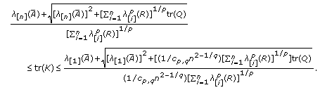  (3.2)

• (2) If , then the trace of matrix has the lower and upper bounds given by

  

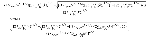  (3.3)

• (3) If , then the trace of matrix has the lower and upper bounds given by

  

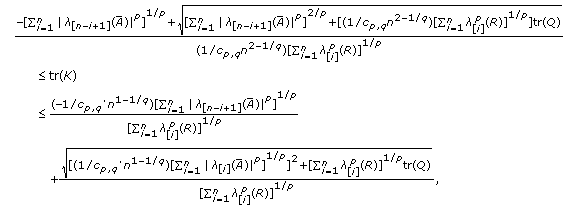  (3.4)

where

(3.5)

Proof.

• (1) Take the trace in both sides of the matrix ARE (1.4) to get

  

  (3.6)

Since is symmetric positive definite matrix, , and from Lemma 2.9, we have

(3.7)

(3.8)

By the Cauchy-Schwartz inequality (2.8), it can be shown that

(3.9)

Note that

(3.10)

, then by (2.34), use (2.6), considering (3.7) and (3.9), we have

(3.11)

From (2.34), note that and then we obtain

(3.12)

It is easy to see that

(3.13)

Combine (3.11) and (3.13), we obtain

(3.14)

Solving (3.14) for yields the right-hand side of the inequality (3.2). Similarly, we can obtain the left-hand side of the inequality (3.2).

• (2) Note that when , and by (2.34), (2.6) and (3.7), we have

  

  (3.15)

Thus,

(3.16)

From (3.11) and (3.16), with similar argument to (1), we can obtain (3.3) easily.

• (3) Note that when , by (3.3), we obtain (3.4) immediately. This completes the proof.

Remark 3.2.

From Remark 2.7 and Theorem 3.1, let in (3.2), then we obtain

(3.17)

where

Remark 3.3.

From Remark 2.7 and Theorem 3.1, let in (3.2), then we obtain (3.1) immediately.

4. Numerical Examples

In this section, firstly, we will give two examples to illustrate that our new trace bounds are better than the recent results. Then, to illustrate the application in the algebraic Riccati equation of our results will have different superiority if we choose different and , we will give two examples when and .

Example 4.1 (see [13] ).

Now let

(4.1)

Neither nor is symmetric. In this case, the results of [6–12] are not valid.

Using (1.9) we obtain

(4.2)

Using (1.11) yields

(4.3)

By (2.18), we obtain

(4.4)

where both lower and upper bounds are better than those of (4.2) and (4.3).

Example 4.2.

Let

(4.5)

Neither nor is symmetric. In this case, the results of [6–12] are not valid.

Using (1.7) yields

(4.6)

From (1.9) we have

(4.7)

Using (1.11) yields

(4.8)

By (1.13), we obtain

(4.9)

The bound in (2.18) yields

(4.10)

Obviously, (4.10) is tighter than (4.6), (4.7), (4.8) and (4.9).

Example 4.3.

Consider the systems (1.1), (1.2) with

(4.11)

Moreover, the corresponding ARE (1.4) with , is stabilizable and is observable.

Using (3.17) yields

(4.12)

Using (3.1) we obtain

(4.13)

where both lower and upper bounds are better than those of (4.12).

Example 4.4.

Consider the systems (1.1), (1.2) with

(4.14)

Moreover, the corresponding ARE (1.4) with , is stabilizable and is observable.

Using (3.1) we obtain

(4.15)

Using (3.17) yields

(4.16)

where both lower and upper bounds are better than those of (4.15).

5. Conclusion

In this paper, we have proposed lower and upper bounds for the trace of the product of two arbitrary real matrices. We have showed that our bounds for the trace are the tightest among the parallel trace bounds in nonsymmetric case. Then, we have obtained the application in the algebraic Riccati equation of our results. Finally, numerical examples have illustrated that our bounds are better than the recent results.

References

Kwakernaak K, Sivan R: Linear Optimal Control Systems. John Wiley & Sons, New York, NY, USA; 1972.
Kleinman DL, Athans M: The design of suboptimal linear time-varying systems. IEEE Transactions on Automatic Control 1968,13(2):150–159. 10.1109/TAC.1968.1098852
Davies R, Shi P, Wiltshire R: New upper solution bounds for perturbed continuous algebraic Riccati equations applied to automatic control. Chaos, Solitons & Fractals 2007,32(2):487–495. 10.1016/j.chaos.2006.06.096
Ni M-L: Existence condition on solutions to the algebraic Riccati equation. Acta Automatica Sinica 2008,34(1):85–87.
Ogata K: Modern Control Engineering. 3rd edition. Prentice-Hall, Upper Saddle River, NJ, USA; 1997.
Wang S-D, Kuo T-S, Hsu C-F: Trace bounds on the solution of the algebraic matrix Riccati and Lyapunov equation. IEEE Transactions on Automatic Control 1986,31(7):654–656. 10.1109/TAC.1986.1104370
Lasserre JB: Tight bounds for the trace of a matrix product. IEEE Transactions on Automatic Control 1997,42(4):578–581. 10.1109/9.566673
Fang Y, Loparo KA, Feng X: Inequalities for the trace of matrix product. IEEE Transactions on Automatic Control 1994,39(12):2489–2490. 10.1109/9.362841
Saniuk J, Rhodes I: A matrix inequality associated with bounds on solutions of algebraic Riccati and Lyapunov equations. IEEE Transactions on Automatic Control 1987,32(8):739–740. 10.1109/TAC.1987.1104700
Mori T: Comments on "A matrix inequality associated with bounds on solutions of algebraic Riccati and Lyapunov equation". IEEE Transactions on Automatic Control 1988,33(11):1088–1091. 10.1109/9.14428
Lasserre JB: A trace inequality for matrix product. IEEE Transactions on Automatic Control 1995,40(8):1500–1501. 10.1109/9.402252
Park P: On the trace bound of a matrix product. IEEE Transactions on Automatic Control 1996,41(12):1799–1802. 10.1109/9.545717
Xing W, Zhang Q, Wang Q: A trace bound for a general square matrix product. IEEE Transactions on Automatic Control 2000,45(8):1563–1565. 10.1109/9.871773
Liu J, He L: A new trace bound for a general square matrix product. IEEE Transactions on Automatic Control 2007,52(2):349–352.
Zhang F, Zhang Q: Eigenvalue inequalities for matrix product. IEEE Transactions on Automatic Control 2006,51(9):1506–1509. 10.1109/TAC.2006.880787
Marshall AW, Olkin I: Inequalities: Theory of Majorization and Its Applications, Mathematics in Science and Engineering. Volume 143. Academic Press, New York, NY, USA; 1979:xx+569.
Wang C-L: On development of inverses of the Cauchy and Hölder inequalities. SIAM Review 1979,21(4):550–557. 10.1137/1021096
Acknowledgments
The author thanks the referee for the very helpful comments and suggestions. The work was supported in part by National Natural Science Foundation of China (10671164), Science and Research Fund of Hunan Provincial Education Department (06A070).
Author information
Authors and Affiliations
Corresponding author
Rights and permissions
Open Access This article is distributed under the terms of the Creative Commons Attribution 2.0 International License (https://creativecommons.org/licenses/by/2.0), which permits unrestricted use, distribution, and reproduction in any medium, provided the original work is properly cited.
About this article
Cite this article
Liu, J., Zhang, J. New Trace Bounds for the Product of Two Matrices and Their Applications in the Algebraic Riccati Equation. J Inequal Appl 2009, 620758 (2009). https://doi.org/10.1155/2009/620758
Received:
Accepted:
Published:
DOI: https://doi.org/10.1155/2009/620758