- Research Article
- Open access
- Published:
Subnormal Solutions of Second-Order Nonhomogeneous Linear Differential Equations with Periodic Coefficients
Journal of Inequalities and Applications volume 2009, Article number: 416273 (2009)
Abstract
We obtain the representations of the subnormal solutions of nonhomogeneous linear differential equation  , where
  and
and  are polynomials in
  such that
  and
and  are not all constants,
  . We partly resolve the question raised by G. G. Gundersen and E. M. Steinbart in 1994.
1. Introduction
We use the standard notations from Nevanlinna theory in this paper (see [1–3]).
The study of the properties of the solutions of a linear differential equation with periodic coefficients is one of the difficult aspects in the complex oscillation theory of differential equations. However, it is also one of the important aspects since it relates to many special functions. Some important researches were done by different authors; see, for instance, [4–9].
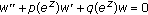
Now, we firstly consider the second-order homogeneous linear differential equations

where  and
and  are polynomials in
  and are not both constants. It is well known that every solution
  of (1.1) is an entire function.
Let  be an entire function. We define

to be the  -type order of
  .
.
If  is a solution of (1.1) and if
  satisfies
  , then we say that
  is a subnormal solution of (1.1). For convenience, we also say that
  is a subnormal solution of (1.1).
-
H.
Wittich has given the general forms of all subnormal solutions of (1.1) that are shown in the following theorem.
Theorem 1 A (see [9]).
If  is a subnormal solution of (1.1), where
  and
and  are polynomials in
  and are not both constants, then
  must have the form

where  is an integer and
  are constants with
  .
.
-
G.
G. Gundersen and E. M. Steinbart refined Theorem A and obtained the exact forms of subnormal solutions of (1.1) as follows.
Theorem 1 B (see [6]).
In addition to the statement of Theorem A, the following statements hold with regard to the subnormal solutions  of (1.1).
(i)If  and
and  then any subnormal solution
  of (1.1) must have the form

where  is an integer and
  are constants with
(ii)If  and
and  , then any subnormal solution
  of (1.1) must be a constant.
(iii)If  , then the only subnormal solution
  of (1.1) is
  .
.
Whether the conclusions of Theorem A and Theorem B can be generalized or not, Gundersen and Steinbart considered the second-order nonhomogeneous linear differential equations

where  , and
, and  are polynomials in
  such that
  are not both constants. They found the exact forms of all subnormal solutions of (1.5), that is, what is mentioned in [6, Theorem ?2.2, Theorem ?2.3 and Theorem ?2.4].
In [6], they also have raised the following problem, that is, what about the forms of the subnormal solutions of the equation

where  , and
, and  are polynomials in
  such that
  ,
,  ,
,  , and
, and  are not all constants?
In [7], we have obtained the exact forms of all subnormal solutions of homogeneous equation

where  , and
, and  are polynomials in
  and are not all constants.
In this paper, we obtain the forms of subnormal solutions of nonhomogeneous linear differential equation (1.6) when  . We have the following theorem.
Theorem 1.1.
Suppose that  is a subnormal solution of (1.6), where
  ,
,  , and
, and  are polynomials in
  such that
  and
and  are not all constants.
(i)If  and
and  , then
  must have the form

where  is a constant,
  and
and  are polynomials in
  .
.
(ii)If  and
and  , then
  must have the form

where  is a constant,
  and
and  are constants that may or may not be equal to zero,
  may be equal to zero or may be a polynomial in
  ,
,  , and
, and  are polynomials in
  with
with  .
.
2. Lemmas for the Proof
In order to prove Theorem 1.1, we need some lemmas.
Lemma 2.1 (see [7]).
Suppose that  is a subnormal solution of (1.7), where
  ,
,  ,
,  and
and  are polynomials in
  and are not all constants.
(i)If  and
and  then any subnormal solution
  must be a constant.
(ii)If  and
and  then
then  must have the form

where  is a polynomial in
  with
with  .
.
Lemma 2.2 (see [10]).
Let  be a transcendental meromorphic function, let
  be a given real constant, and let
  . Then there exists a constant
  such that the following two statements hold (where
  ).
).
(i)There exists a set  that has linear measure zero such that if
  , then there is a constant
  such that for all
  satisfying
  and
and  one has

(ii)There exists a set  that has finite logarithmic measure such that (2.2) holds for all
  satisfying
  .
.
Lemma 2.3 (see [6]).
Let  with
with  as
as  and let
  Let
Let

and set

Let  be analytic on the set
  . Suppose that
  is unbounded on the set
  . Then there exists an infinite sequence of points
  with
with  as
as  such that

Lemma 2.4 (see [8]).
Consider the nth- order differential equation of the form

where  are polynomials in
  and
and  with
with  . Suppose that
  is an entire and subnormal solution of (2.6) and that
  can be expressed as
  , where
  is a constant and
  is analytic on
  . Then
  has the form

where  is a constant and
  and
and  are polynomials in
  .
.
As an application of Lemma 2.4, one has the following lemma.
Lemma 2.5.
Suppose that  is an entire subnormal solution of (2.6), where
  are polynomials in
  and
and  with
with  , and that
  and
and  are linearly dependent. Then
  has the form

where  is a constant and
  and
and  are polynomials in
  .
.
Proof.
Since  is entire and is linearly dependent with
  ,
,  can be written as
  (see [11, page 382]), where
  is a constant and
  is analytic on
  . Then we have the representation from Lemma 2.4.
Lemma 2.6.
Suppose that  is a solution of (1.6), where
  ,
,  ,
,  ,
,  ,
,  , and
, and  are polynomials in
  such that
  ,
,  ,
,  and
and  are not all constants. If

then there exists a polynomial  such that

where  is a solution of

where  and
and  are polynomials in
  with
with 
Proof.
Let  and set

where  is the constant such that

It follows from (1.6) and (2.12) that

where

So  and
and  are polynomials in
  and
and  , respectively, and
  by (2.13), but
  and
and  have the exact representations that depend on the relations of
  , and
, and  . If
. If  , then (2.14) is of the form (2.11), and (2.12) gives (2.10). If
  , then we repeat the above process finite times until we obtain (2.10) and (2.11). This completes the proof of Lemma 2.6.
3. Proof of Theorem
In this section, we will prove Theorem 1.1.
Proof.
-
(i)
Suppose that
 is a subnormal solution of (1.6) with
  and
and  . If
. If  is a polynomial solution of (1.6), then
  must be a constant, which is of the form (1.8). Thus we suppose that
  is transcendental. It follows from Lemma 2.2(i) that there exists a set
  that has linear measure zero such that if
  , then there is a constant
  such that for all
  satisfying
  and
and  , we have
 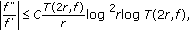 (3.1)
(3.1)
 is a subnormal solution of (1.6) with
  and
and  . If
. If  is a polynomial solution of (1.6), then
  must be a constant, which is of the form (1.8). Thus we suppose that
  is transcendental. It follows from Lemma 2.2(i) that there exists a set
  that has linear measure zero such that if
  , then there is a constant
  such that for all
  satisfying
  and
and  , we have
where  is a constant and
  . It also follows from Lemma 2.2(ii) that there exists a set
  that has finite logarithmic measure such that (3.1) holds for all
  satisfying
  .
.
Now let  be an infinite sequence satisfying
  such that
  for all
  and
and  as
as  Let
Let  be a small constant such that
  and
and  . Set
. Set

and set

From above, we have that (3.1) holds on the set 
We now assert that  is bounded on the set
  . On the contrary, it follows from Lemma 2.3 that there exists a sequence of points
  with
with  as
as  such that


By (1.6), we have for all  ,
,

It follows from (3.4)–(3.6) and  that (3.6) yields
  as
as  on the set
  This is a contradiction.
By the maximum modulus principle,  is bounded in the angular domain

However, we know

where the integral of  is defined on the simple contour
  , extending from a point
  to a point
  in the complex domain.
So we obtain

as  in the angular domain
  .
.
Thus , from the Cauchy integral formula, we obtain

as  in the angular domain
  . By (1.6), (3.8), and (3.9), we have for some constant

as  in the angular domain
  . Together with (3.8) and (3.11),
  is bounded in the angular domain
  .
.
If  , it follows from Lemma 2.5 that
  must have the form (1.8).
If  , since
  is a subnormal solution of (1.6), so is
  . Thus,

will be a subnormal solution of (1.7). Since we suppose that  , we will discuss the following two cases.
Case 1.
If  we have, by Lemma 2.1(i),

where  is a constant. Hence
  , that is,

From this,  can be written as
  (see [11, page 382]), where
  is a constant and
  is analytic on
  . Thus,
  can be written as
  , where
  is a constant and
  is analytic on
  . It follows from Lemma 2.4 that

where  is a constant,
  and
and  are polynomials in
  . Thus,
  has the form of (1.8).
Case 2.
If  we obtain from Lemma 2.1(ii) that

where  is a polynomial in
  with
with  .
.
However, we can assert that  in (3.16). Otherwise, there exists
  such that

By (3.16), we have

Thus from (3.16) and (3.18), we have

By repeating this process finite times, we obtain that for any integer  ,
,

We have, by (3.17) and (3.20),

as  This is a contradiction to the fact that
  is bounded in the angular domain
  . This shows that
  is not possible when
  under the hypotheses. This completes the proof of part (i).
-
(ii)
We firstly suppose that
 . Since
  is a subnormal solution of (1.6), so is
  . Set
. Set 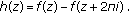 (3.22)
 . Since
  is a subnormal solution of (1.6), so is
  . Set
. Set 
Then  is a subnormal solution of (1.7). Now if
  , this shows that
  and
and  has the form of (1.9) by Lemma 2.5. Thus, we suppose that
  in the following.
Now, assume that  .
.
If  it follows from the proof of Case 1 of Theorem 1.1(i) that
  has the form of (1.9).
If  we obtain from Lemma 2.1(ii) that

where  is a polynomial in
  with
with  .
.
Set

where  is an integer and
  are constants with
Let  and set

where 
Now, we will discuss the following two cases.
Case A.
We consider  in (3.24). Let
  be a constant defined by

and set

Since  is a subnormal solution of (1.7), it follows from (3.27) that
  satisfies

We obtain from (3.23)–(3.28) that

where  and
and  are polynomials in
  with
with 
Set

It follows from (1.6), (3.25), (3.29) and (3.30) that 
Set

So  , and
, and  satisfies

We have by (3.27) that  is a subnormal solution of (1.7),
  is a subnormal solution of (3.29). Moreover,
  is also a subnormal solution of (3.32) by (3.30) and
  is a subnormal solution of (1.6). Thus, we deduce from Theorem 1.1(i) and (3.32) with
  that
that  has the form

where  is a constant,
  and
and  are polynomials in
  . Hence (3.23), (3.24), (3.27), (3.30), and (3.33) yield

where  and
and  are constants,
  , and
, and  are polynomials in
  with
with  . This is the form of (1.9).
Case B.
We consider  in (3.24). Let
  be a constant defined by

where  is a number such that
  is the first coefficient
  in (3.24) which is not equal to zero. Set

Similar to the proof of Case A of Theorem 1.1(ii), we have

where  and
and  are constants,
  and,
and,  are polynomials in
  with
with  . Set
. Set  . Then
  is a polynomial in
  by the hypotheses of
  in (3.36). This is the form of (1.9). We have proved Theorem 1.1(ii) when
Now we suppose that  . By Lemma 2.6, there exists a polynomial
  in
in  , satisfies (2.10) and (2.11).
Since  and since we have proved Theorem 1.1 holds in the cases when
  holds, we can apply this result to (2.11).
If  , it follows from Theorem 1.1(i) that

where  is a constant,
  and
and  are polynomials in
  . By (2.10) and (3.38), we obtain that

where  is a constant,
  and
and  are polynomials in
  . This is a form of (1.9).
If  , it follows from the proof of Theorem 1.1(ii) when
  that
that

where  and
and  are polynomials in
  with
with  ,
,  and
and  are constants that may or may not be equal to zero. By (2.10) and (3.40), we obtain that
  has the form of (1.9). Theorem 1.1(ii) is completed.
Now, we give some examples to show that Theorem 1.1 is correct.
Example 3.1.
Let  , then
  satisfies

This is an example of Theorem 1.1(i).
Example 3.2.
Let  , then
  satisfies

This is an example of Theorem 1.1(ii) with  and
and  .
.
Example 3.3.
Let  , then
  satisfies

This is an example of Theorem 1.1 (ii) with  and
and  .
.
References
Gao SA, Chen ZX, Chen TW: Oscillation Theory of Linear Differential Equation. Huazhong University of Science and Technology Press; 1998.
Hayman WK: Meromorphic Functions, Oxford Mathematical Monographs. Clarendon Press, Oxford, UK; 1964:xiv+191.
Yang L: Value Distribution Theory and Its New Researches. Science Press, Beijing, China; 1992.
Chen ZX, Shon KH: On subnormal solutions of second order linear periodic differential equations. Science in China. Series A 2007,50(6):786–800. 10.1007/s11425-007-0050-3
Chen ZX, Gao SA, Shon KH: On the dependent property of solutions for higher order periodic differential equations. Acta Mathematica Scientia. Series B 2007,27(4):743–752. 10.1016/S0252-9602(07)60072-1
Gundersen GG, Steinbart EM: Subnormal solutions of second order linear differential equations with periodic coefficients. Results in Mathematics 1994,25(3–4):270–289.
Huang ZB, Chen ZX: Subnormal solutions of second order homogeneous linear differential equations with periodic coefficients. Acta Mathematica Sinica, Series A 2009,52(1):9–16.
Urabe H, Yang CC: On factorization of entire functions satisfying differential equations. Kodai Mathematical Journal 1991,14(1):123–133. 10.2996/kmj/1138039342
Wittich H: Subnormale Lösungen Differentialgleichung:
 Nagoya Mathematical Journal 1967, 30: 29–37.
Gundersen GG: Estimates for the logarithmic derivative of a meromorphic function, plus similar estimates. Journal of the London Mathematical Society 1988,37(1):88–104.
Ince E: Ordinary Differential Equations. Dover, New York, NY, USA; 1926.
 Nagoya Mathematical Journal 1967, 30: 29–37.
Acknowledgements
The authors are very grateful to the referee for his (her) many valuable comments and suggestions which greatly improved the presentation of this paper. The project was supposed by the National Natural Science Foundation of China (no. 10871076), and also partly supposed by the School of Mathematical Sciences Foundation of SCNU, China.
Author information
Authors and Affiliations
Corresponding author
Rights and permissions
Open Access This article is distributed under the terms of the Creative Commons Attribution 2.0 International License ( https://creativecommons.org/licenses/by/2.0 ), which permits unrestricted use, distribution, and reproduction in any medium, provided the original work is properly cited.
About this article
Cite this article
Huang, ZB., Chen, ZX. & Li, Q. Subnormal Solutions of Second-Order Nonhomogeneous Linear Differential Equations with Periodic Coefficients. J Inequal Appl 2009, 416273 (2009). https://doi.org/10.1155/2009/416273
Received:
Accepted:
Published:
DOI: https://doi.org/10.1155/2009/416273